The LCGC Blog: The Beauty of the Quadrupole Mass Analyzer
The quadrupole mass analyzing device is now accessible to many analytical chemists as a detector in either HPLC or GC instruments due to their increasingly accessible price point. While it’s not vital that we understand the working principle of these detectors, insight into their design and operation can help enormously when planning or optimizing analyses or troubleshooting issues. Warning: there are equations in this blog. Embrace your inner physicist. To properly understand the quadrupole principles, you need to have an appreciation of the underlying mathematics.
Quadrupole mass analyzers were first described and developed in 1953 by West German physicists Wolfgang Paul and Helmut Steinwedel while they were working at the University of Bonn. In this detector device, electric fields are used to separate ions according to their mass-to-charge ratio (m/z), the ratio of mass in daltons (Da) to the integer number of charges (z), as they pass along the central axis of parallel and equidistant poles or rods. Each rod has two voltages applied, one of which is a fixed direct current (DC) and the second is an alternating current (AC), that cycles with a superimposed radio frequency (in MHz frequency domain).
The magnitude of the applied electric field can be ordered such that only ions with a specific m/z value can travel through the quadrupole, prior to being detected. Ions with all other m/z values are deflected onto trajectories that would cause them to collide with the quadrupole rods and discharge or be ejected from the mass analyzer field and removed via the vacuum. The quadrupole is often referred to as an exclusive detector because only ions with a specific m/z are stable in the quadrupole at any one time, according to the applied voltages. Those ions with a stable trajectory are often referred to as having non-collisional, resonant, or stable trajectories.
A typical quadrupole mass analyzer consists of four rods with a hyperbolic internal cross-section. The quadrupole rods are typically constructed using molybdenum alloys because of their inherent inertness and lack of activity. Very high degrees of accuracy and precision (in the micrometer region) in rod machining and relative positioning are required to achieve unit mass accuracy (Figure 1). For clarity, the figure shows the rods with a much smaller diameter than in reality.


Figure 1: Schematic diagram showing the construction and applied voltages for a typical quadrupole mass analyzing device. Note the rod diameter in the schematic is not to scale and is smaller than in the real-life detector.
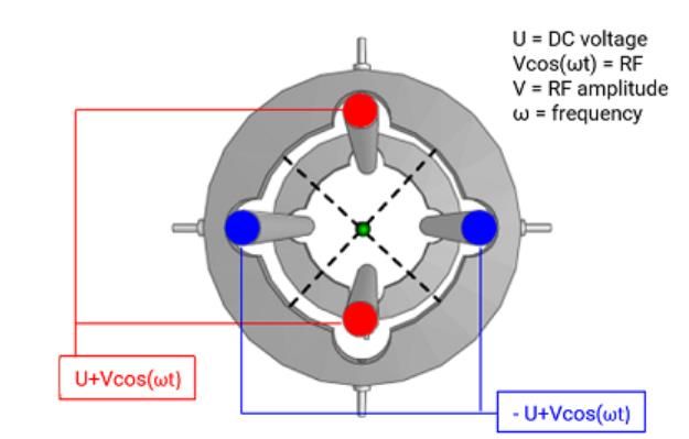
It is a common misconception that the quadrupole mass analyzer consists of a pair of constantly positive and negative rods. Because of the alternating voltage (V), oscillating at a radio frequency (commonly called the "RF voltage", whose frequency is described by cosine ωt), each pair of rods will be successively positive, then negative, and so forth. In essence, there will always be a pair of more positive and more negative rods, however, they will alternate positive and negative at the radio frequency. The misnomer arises as one rod pair has a negative direct current (DC) voltage offset (-U) and the other a positive DC offset voltage (+U). Figure 2 shows the relationship between the voltages of the red and blue rods of the quadrupole from Figure 1.


Figure 2: Magnitude and phasing of the rod voltages form the quadrupole shown in Figure 1.

Note from Figure 2 that each rod pair cycles through both positive and negative total applied voltage, but they are differently “offset” in either the positive or negative direction by +U and -U (the so-called DC voltage) respectively and the total applied voltage is out of phase between each rod pair by 180o.
Application of voltages on the quadrupole rods creates a hyperbolic field in the central space defined by the outer surfaces of the rods, which can be defined by Equation 1 (the Laplace Equation), and the resulting overall field created is shown in Figure 3.
Equation 1:


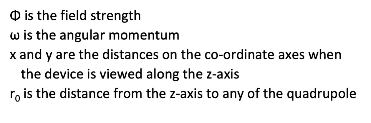


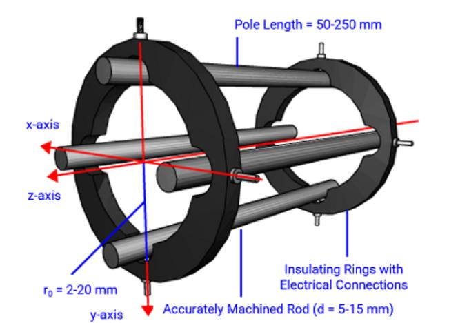

 and the resulting field created within the so-called \"tunnel\" radius in the central space between the rod surfaces (2r0). Note the rod diameter in the schematic is not to scale and is smaller than in the real-life detector.")
Figure 3: Quadrupole image demonstrating the various dimensions from Equation 1 (top) and the resulting field created within the so-called "tunnel" radius in the central space between the rod surfaces (2r0). Note the rod diameter in the schematic is not to scale and is smaller than in the real-life detector.
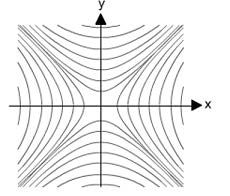
When x = y, Φ =0 giving rise to planes of zero-field strength within the quadrupole. At all other positions between the poles, the oscillating electric field (Φ) causes ions to be alternately attracted to and repelled by the pairs of rods. Note that Equation 1 shows that the field has no effect along the direction of the central (z) axis within the quadrupole and so to facilitate the passage of ions through the mass analyzer an accelerating voltage is applied across the mass analyzer to enable ions to move through the device.
An ion traveling through the quadrupole will successively be attracted and then repelled from each rod until it describes what is known as a "saddle" field. The positive analyte ion is initially attracted by negative rods and acquires some kinetic energy. However, the polarity of the voltage quickly switches, and the Kinect energy is converted to potential energy and is “repelled” back into the center space of the quadrupole. To visualize this, think of a tennis ball at rest on a horse saddle. Nudging the ball will cause it to fall down the sides of the saddle. However, if we quickly rotate the saddle 90o, the ball will encounter an upward facing surface and will move towards its original position. The field experienced by the ion will be equivalent to the motion described if the saddle were rotated at high speed, successively falling and then moving back to its original position or riding on the upward-facing surfaces.
Heavy ions are less affected by the alternating current (V) and respond to the average voltage within the space within the quadrupole, focusing them towards the center of the rods. Lighter ions respond more readily to the alternating current and may have an unstable trajectory in the Y-Z plane of Figure 1 and will not reach the detector. Only ions heavier than a selected mass will not be filtered out by the Y-Z (positively biased) rods and as such these rods are known as a high pass mass filter. The rods in the X-Z plane have a negative DC voltage offset and heavy ions are still most affected by the DC potential, but since it is negative, they strike the rod and are unable to reach the detector. The lighter ions respond to the AC potential and are focused towards the center of the quadrupole. The AC potential can be thought of as correcting the trajectories of the lighter ions, preventing them from striking the rods in the X-Z plane and therefore these rods are known as a low pass mass filter.
When the ion is caused to oscillate with a trajectory whose amplitude exceeds r0 it will collide with a rod and discharge or pass out of the mass analyzer without being detected (non-resonant, unstable, or collisional trajectory).
The trajectories described for the ions through the quadrupole are complex and cannot be described in a simple way because they include a large number of physical variables that affect the instantaneous electric fields experienced by the ions, however, I have attempted to show a resonant and non-resonant trajectory in schematic form in Figure 4.

 and the green path is non-resonant (unstable).")
Figure 4: Schematic representations of the ion movement within a quadrupole. The path described by the red line is resonant (stable) and the green path is non-resonant (unstable).

Using the Laplace Equation (Equation 1), the following relationships can be derived to represent the acceleration of ions within the quadrupole saddle field:


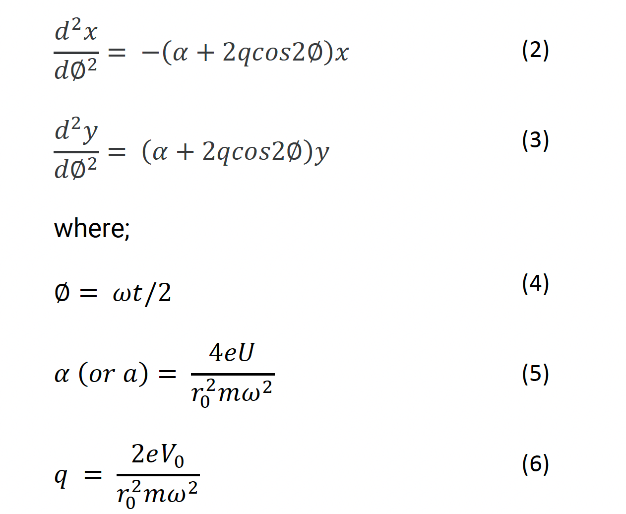
e – is the charge on the ion, m – is the mass of the ion
You will notice from Equations 2 and 3 that the acceleration of an ion in either the x or y plane is proportional to a(a) or q. In turn, a is proportional to U/m (Equation 5) and q is proportional to V0/m (Equation 6). We now have a relationship between the two applied voltages and the acceleration of ions within the electrostatic field within the quadrupole.
Thus, for any particular ion of m/e (more correctly written as m/z), the position of the ion within the quadrupolar field is dependent upon U, V, ω, e and r0. Because, ω, e and r0 are either fixed (ω, r0) or a simple constant integer value (e), varying values of U and V will cause ions move according to the applied saddle field. Proving the ions deflection in the x and y-axis, which determines its position from the center of the rod cluster, remain less than r0, the ion will pass through the quadrupole without touching the rods or being lost from the device to the vacuum (resonant, non-collisional, or stable trajectory).
The relationship between the DC and AC (RF) voltages and the mass-to-charge ratio of stable ions can be plotted on a Mathieu diagram using equations 4 and 5.

 and q (V0) for an ion of particular m/z value or range of values. The call-out box shows the regions of a and q (U and V) values which are typically used in mass spectrometers for analytical chemistry.")
Figure 5: Mathieu diagrams showing the stable combinations of a (U) and q (V0) for an ion of particular m/z value or range of values. The call-out box shows the regions of a and q (U and V) values which are typically used in mass spectrometers for analytical chemistry.
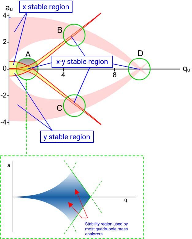
Figure 5 shows the region of a(U) and q(V0) values which are used in quadrupole mass filters familiar to analytical chemists. But how do we relate the mass of the ions we are separating and detecting to the values of U and V and therefore to the ratios of DC and AC voltages that we need to apply to the quadrupole to ensure a stable trajectory for an ion of a particular mass? Figure 6 can help us to understand this further.

 and q (V0) for an ion of mass 219 and charge 1. The red line shows a SCAN function and the region of the scan demarked by the double-headed arrow shows the range of U and V values (held in a constant ratio) which result in unit mass resolution for Mass 219.")
Figure 6: Mathieu diagrams showing the stable combinations of a (U) and q (V0) for an ion of mass 219 and charge 1. The red line shows a SCAN function and the region of the scan demarked by the double-headed arrow shows the range of U and V values (held in a constant ratio) which result in unit mass resolution for Mass 219.
Any value of U and V bounded by (lying within) the blue region within the stability diagram will pass through the quadrupole with a stable trajectory and therefore will reach the detector. In Figure 6, the diagram represents the stable region for an ion of mass 219Da and unit charge. By setting the values of U and V to the point represented by "m" on the figure, the mass analyzer will have unit mass resolving power, meaning 219 ± 0.5Da. This represents a Selected Ion Monitoring (SIM) experiment in which the values of U and V and fixed to allow a selected target mass to pass through the filter while all other masses are lost on unstable trajectories.
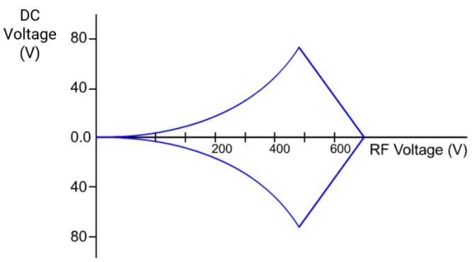
The values of U and V may also be varied in a constant ratio as demonstrated by the red line in Figure 5. This allows the quadrupole to SCAN through a range of masses, each of which will be subsequently allowed to pass through the mass analyzer to the detector. This principle is demonstrated in Figure 7 which shows three selected target tune masses associated with perfluorotributylamine (PFTBA), a popular tune compound used with Gas Chromatography-Mass Spectrometers (GC-MS).

 allows ions of increasing mass to momentarily pass through the detector.")
Figure 7: Quadrupole scanning, in which values of U and V are held in a constant ratio with magnitude varying according to the solid line in the top diagram. The scanning through the applied voltage range (typically from high to low values) allows ions of increasing mass to momentarily pass through the detector.

Figure 7 shows the SCAN line function that allows a pre-defined range of masses to be sequentially monitored using a quadrupole mass filter, by varying the magnitude of U and V over a range value while holding the ratio of U/V constant. The Figure indicates three tune masses and their respective Matthieu stability curves, however, it should be noted that all other mass between those shown will also be included in the scan function, provided that some values of U/V on the SCAN line fall with their stability curve. This allows the user to set a can “range” of mass values through which the instrument will sequentially move and to record the presence of any ions within this mass range in a single scanning experiment that will typically be achieved at a frequency of several Hz depending upon the magnitude of the mass range selected, wider mass ranges taking longer to scan and therefore reducing the scanning frequency.
Two important factors shown in Figure 7 are the "U offset" value and the "gain" or slope of the SCAN function line. These two parameters are typically available as variables to the user and can be used to “tune” the sensitivity and resolution of the mass analyzer. As one reduces either the offset or gain, the abundance of the number of ions passing through the detector is increased. Think of this as the total area under the Matthieu curve t is bisected by the SCAN function line. As we decrease the quadrupole gain, the resolution of the instrument will decrease, but the sensitivity will increase (total area under the curve defined by the scan line). The opposite is also true in respect of increasing the quadrupole gain or offset, sensitivity will decrease, and resolution will increase. These concepts are further explained in Figure 8, and the manipulation of the gain and offset parameters are often used to tune the mass spectrometer devices during an autotune routine and can also be used to improve sensitivity of the instruments, for target masses or mass ranges, by the user.

 and offset (y-intercept) of the quadrupole scan function in order to alter the sensitivity and resolution of the mass analyzer")
Figure 8: Varying the Gain (slope) and offset (y-intercept) of the quadrupole scan function in order to alter the sensitivity and resolution of the mass analyzer

At the start of this blog, I mentioned that it was not important to understand the fundamentals of the mass analyzer in order to produce data, and this is true. However, I remember my own reaction when I was first taught the underlying principles of the quadrupole device and the sheer “game-changing” nature of its effect on my abilities with chromatography using MS detection. I can’t expect this simple treatment to have had the same effect, but if you get the opportunity, ask someone to show you the effects of changing gain and offset on a quadrupole and assess just how the instrument response fits perfectly with the operational theory. Perhaps then you will have a similar attitude to the sheer beauty of these mass analyzing devices!


Tony Taylor

Tony Taylor is the Chief Scientific Officer of Arch Sciences Group and the Technical Director of CHROMacademy. His background is in pharmaceutical R&D and polymer chemistry, but he has spent the past 20 years in training and consulting, working with Crawford Scientific Group clients to ensure they attain the very best analytical science possible. He has trained and consulted with thousands of analytical chemists globally and is passionate about professional development in separation science, developing CHROMacademy as a means to provide high-quality online education to analytical chemists. His current research interests include HPLC column selectivity codification, advanced automated sample preparation, and LC–MS and GC–MS for materials characterization, especially in the field of extractables and leachables analysis.
 and is based in New Jersey, USA. He earned his two B.S. degrees at the University of Arizona and his Ph.D. in Chemistry from the University of Michigan under the direction of Prof. Robert T. Kennedy. Prior to joining BMS, he held a National Research Council position at the National Institute of Standards and Technology (NIST) and was a professor of chemistry at Temple University in Philadelphia, PA. To date he has authored more than 40 manuscripts and two book chapters. He has presented more than 40 oral or poster presentations and holds one patent in the field of separation science. Jonathan has proudly served on the executive board of the ACS Subdivision on Chromatography and Separations Chemistry (SCSC) for three terms.")


The LCGC Blog, Paying it Forward: Perspectives from a Fulbright–Palacky Distinguished Scholar
January 5th 2024In this LCGC Blog, Kevin Schug shares his plans for the future as a Fulbright–Palacky University Distinguished Scholar in the Czech Republic, and discusses why it is important to share analytical chemistry with communities around the world.