Are You Ready to Switch to Comprehensive Two-Dimensional Gas Chromatography?

In the past two decades, comprehensive two-dimensional gas chromatography (GC×GC) has progressed from an interesting concept to the forefront of thinking and research in gas chromatography. Especially when combined with mass spectrometry detection, GC×GC provides high resolution, high sensitivity, and massive chromatographic data sets, which is useful in diverse fields such as petroleum analysis, metabolomics, food, flavor, fragrance, and environmental analysis. In this installment, recent developments in GC×GC that make it more amenable for routine use are discussed. These include advances in instrumentation, especially modulation, column sets, data analysis, and the range and types of samples amenable to GC×GC. We will ponder the question – are you ready to make the switch to GC×GC?

Comprehensive two-dimensional gas chromatography (GC×GC) was developed in the 1990s in the laboratory of the late Professor John Phillips at Southern Illinois University (1). A book chapter by Dimandja provides an excellent overview of the development of GC×GC in the Phillips lab (2). Dimandja traces the development of coupled columns in GC, in which columns of differing stationary phase chemistries are connected in tandem, from simple coupling of columns to heart-cutting to comprehensive GC×GC. The goal of any chromatographic technique involving multiple stationary phases in the same separation is to achieve a desired selectivity.

When two capillary columns of differing stationary phases are connected in tandem, there are three possibilities, as summarized in Table I. If the columns are simply connected end-to-end, the final selectivity will be a combination of the selectivity of the two initial columns. If the two columns are of equal dimensions, they will roughly contribute equally to the selectivity of the final separation. A second possibility is to add a simple switching valve at the outlet of the first column that directs a portion of the effluent, such as one peak, or a timed portion, into the second column. This is called heart-cutting and allows the second stationary phase to separate a small set of analytes not separated on the first. If heart-cutting is extended to its limit, sampling the first column effluent continuously every few seconds, then assembling each short cut or slice into a three-dimensional plot, we obtain GC×GC.

TABLE I: Summary of tandem column configurations

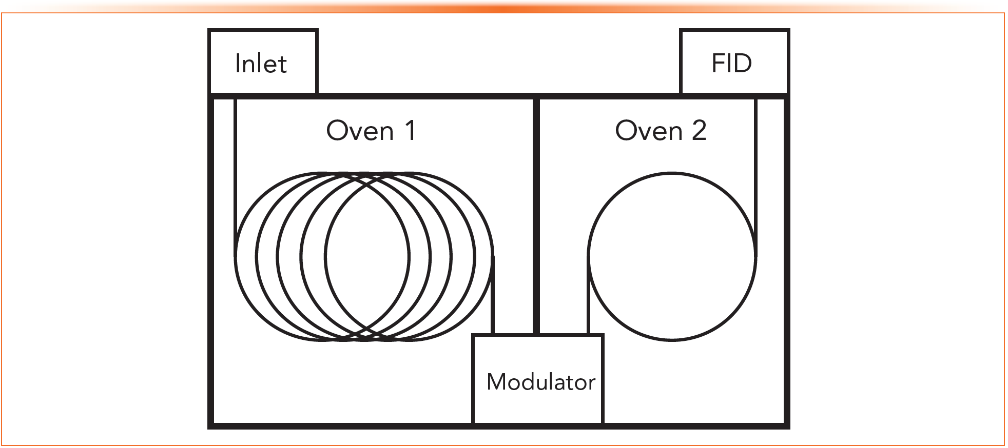
Figure 1 shows a simplified instrumental diagram of a tandem column system. The device connecting the two columns is called a modulator. In GC×GC, the two columns are usually housed in separately controlled column ovens, although this is not always required. Tandem columns provide an advantage of allowing a multidimensional separation using a single detector. With the timing of each slide being carefully controlled, a single chromatogram is generated. The data system then slices the single plot into each short second-dimension slice and aligns the slices into a single plot with the two separation dimensions as the x- and y-axes and the signal intensity as the z-axis.

FIGURE 1: Diagram of a tandem-column multidimensional gas chromatograph. The modulator can be any of the configurations described in Table I.

The Modulator

If the column is considered the heart of a one-dimensional separation rather than the modulator, a device that both connects the columns and transfers the first-dimension column effluent into the second-dimension column effluent will act as the heart of multidimensional chromatography. Like the inlet on a traditional gas chromatograph, the modulator must collect a chosen aliquot of the first-dimension effluent, focus it into a very narrow band at the head of the second column and then inject it rapidly into the second column. Keep in mind that in GC×GC the second column is usually very short, 1–2 meters long, with retention times measured in a few seconds.

There are three types of modulators used for GC×GC, thermal, valve, and flow, with thermal and flow being most used in commercial systems. Each has advantages and disadvantages that relate to both analytical performance and ease of use. Figure 2 shows a diagram of the steps involved with a thermal modulator, which is easy to understand and illustrates the steps needed to ensure that the effluent is efficiently transferred between the two columns, while preventing carryover from one second-dimension injection into the next.

FIGURE 2: Schematic of the cryotrap modulator and peak modulation process: (a) first cold jet focuses peak of single component; (b) first hot jet moves peak to second cold jet; (c) second cold jet splits peak of component; and (d) second hot jet moves peaks for component into secondary oven.

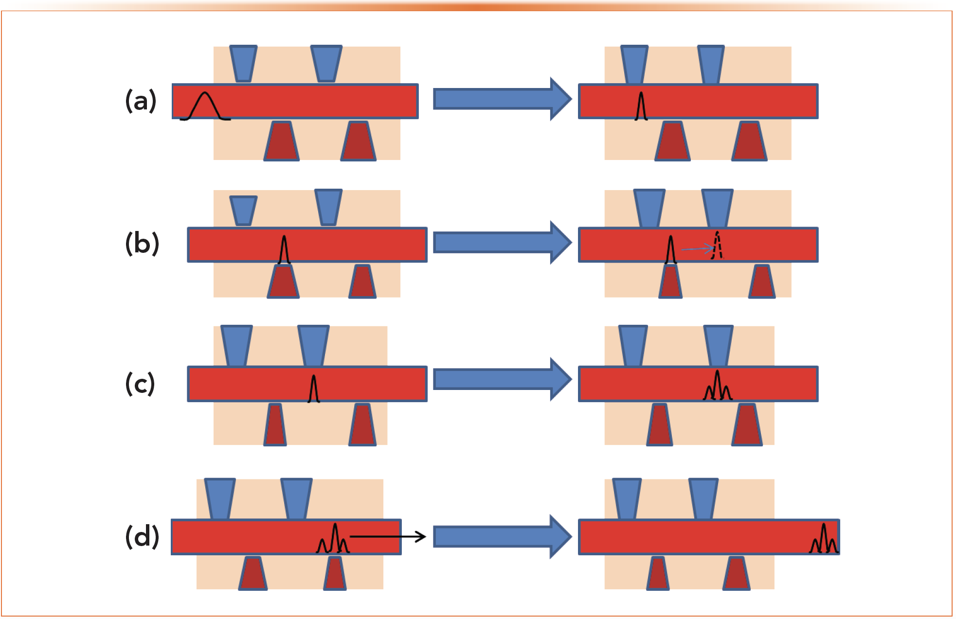
This thermal modulator uses two cold jets and two hot jets that operate in sequence to transfer the sample. Typically, the cold jets employ liquid nitrogen, and the hot jets employ nitrogen gas. One obvious disadvantage of thermal modulation is the need for cryogens to provide the best peak focusing. The first cold jet activates and traps the analytes in a narrow band. This is followed by the first hot jet activating and rapidly transferring the analytes to the second stage, where the second cold jet activates and traps them in a narrow band. The first cold jet then re-activates to trap the next analyte band, while the second hot jet injects the first band into the second column.

This process illustrates the basic principles for all modulators, transferring the analytes from the first column to the second in repeating, reproducible narrow bands, with no bleed or carryover between slices. The need for no carryover is why modulators generally have two stages. Analytes exiting from the first column are stopped while injection into the second column is happening.

Advances in Data Analysis

Not surprisingly, data sets in GC×GC and especially GC×GC–MS are quite large and include many levels of information, including first- and second-dimension retention times, peak widths, peak height, peak area, peak shape in both dimensions, and, if using MS, a full mass spectrum of each peak. In many untargeted situations, this can mean hundreds of peaks and mass spectra in a single analysis. With such large data sets, automated chemometric techniques are needed. If a chromatogram is seen as a fingerprint of a sample, think about the complexities involved if two or more are to be compared, now in multiple dimensions and with a spectrometric detector, such as a mass spectrometer, providing yet another data dimension.

There are several statistical techniques for both qualitative and quantitative comparison of these complex multidimensional chromatograms that perform basic functions: i) deconvolution, in which the individual signals that generate unseparated peaks can be separated; ii) qualitative and quantitative pattern recognition, in which compounds of interest are identified and quantified, likely among large numbers of peaks that are not of interest. Berrier, Prebihalo and Synovec introduced the basics of these techniques, many of which are available as components of commercial data systems for GC×GC (3).

Most recently, chromatogram tiling has become available, in which pattern recognition is performed by separating the larger two-dimensional chromatogram into smaller tiles, accounting for small variations in retention times in both dimensions and aligning the chromatograms for component identification and pattern recognition (4). The best way for a new user to distinguish between and choose the necessary techniques is to discuss their needs and possibilities in detail with instrument vendors’ technical support teams.

When Should I Use GC×GC?

There are several considerations in making a transition from GC to GC×GC, with situations in both targeted and untargeted analyses lending themselves to GC×GC, with some specific cases in petroleum and drug analysis having been discussed in a previous column (5). The utility of GC×GC in untargeted analysis is straightforward. We want to see as many components in the mixture as possible and may be concerned with the identity of some or all of them. This started with petroleum and related analyses and has moved to metabolomic studies in clinical, pharmaceutical, food, environmental, and other situations where there are complex mixtures and all the peaks may be of interest. In many of these cases, there may be many samples with large numbers of analytes in each one that may not all be the same. GC×GC, especially GC×GC–MS lends itself well to this situation.

In targeted analysis, we either have many specific analytes that need to be identified or quantified, or a small number of analytes mixed with a complex sample matrix. GC×GC and GC×GC–MS also lend themselves well to these situations. If there are many possible analytes to quantify in a single method, such as in drug testing or pesticide analysis, GC×GC allows for more separation space, and more potentially fully-separated peaks can fit into the space of one chromatogram. In pharmaceutical residual solvents analysis, there are more than 50 possible analytes, but only a few of them may be present in any single analysis. However, the method must still account for fully separating all of them, with required selectivity stated by regulatory bodies (6). Figure 3 shows a contour plot chromatogram of pharmaceutical residual solvents, illustrating the power of GC×GC for targeted analysis. Each analyte is represented as a bright spot against the blue background of the baseline. The specific analytes are listed in the reference.

FIGURE 3: Two-dimensional chromatogram of 58 pharmaceutical solvents, showing multiple selectivities possible in GC×GC. Reprinted from reference (6) with permission from the author.

Figure 3 also illustrates the power of GC×GC to separate analytes from matrix components. In this example, the analytes were dissolved in methanol, which shows up as a large peak to the left in the chromatogram. Note that the methanol peak shows tails in both dimensions, seen as stripes moving up and to the right from the main peak. With the second-dimension separation, the analyte peaks are separated from the methanol peak tails. In a traditional one-dimensional separation, the analyte peaks would lie on top of the methanol peak tail, potentially impacting the baseline and integration of the analyte peaks.

Finally, note that this chromatogram is presented roughly as a square contour plot, yet the x-axis time is in minutes and the y-axis is in seconds. While this makes it easier to visualize the peaks, be aware that the actual chromatogram, if drawn to scale, would look like a narrow strip, not a square.

Conclusion

GC×GC and GC×GC–MS have come a long way in the last several years. With increasingly robust modulators and advanced data handling capabilities, application has expanded well beyond its roots in petroleum-related analysis to nearly all fields in which complex mixtures are separated or where individual analytes may be separated from complex matrices. For new users, the best way to consider transitioning into GC×GC is the same as with any new instrument: Carefully outline the problem and scientific questions you are working to solve, then explore possible solutions with the scientific literature and instrument vendors. In the GC×GC space, which remains somewhat specialized, vendors are an excellent place to start.

References

(1) Bode, G. His opponents were in for a challenge when they faced John Phillips in a game of Scrabble. He had a habit of plunking down tiles to form words they did not recognize, only to prove to protesters who brought out the dictionary the words really existed. The Daily Egyptian, 1999. https://dailyegyptian.com/40529/archives/his-opponents-were-in-for-a-challenge-when-they-faced-john-phillips-in-a-game-of-scrabble-he-had-a-habit-of-plunking-down-tiles-to-form-words-they-did-not-recognize-only-to-prove-to-protesters-who-b/ (accessed 2023-08-01).

(2) Dimandja, J. Introduction and Historical Background. In Basic Multidimensional Gas Chromatography, 1st ed.; Elsevier, 2020, 1–40.

(3) Berrier, K. L.; Prebihalo, S. E.; Synovec, R. E. Advanced Data Handling in Comprehensive Two-dimensional Gas Chromatography. In Basic Multidimensional Gas Chromatography, 1st ed.; Elsevier, 2020, 229–268.

(4) Cain, C. N.; Trinklein, T. J.; Ochoa, G. S.; Synovec, R. E. Tile-Based Pairwise Analysis of GC×GC–TOF-MS Data to Facilitate Analyte Discovery and Mass Spectrum Purification. Anal. Chem. 2022, 94 (14), 5658–5666. DOI: 10.1021/acs.analchem.2c00223

(5) Snow, N. H. GC×GC: From Research to Routine. LCGC N. Am. 2019, 37 (2) 92–101, 130.

(6) Crimi, C. M.; Snow, N. H. Analysis of Pharmaceutical Residual Solvents Using Comprehensive Two-dimensional Gas Chromatography. LCGC N. Am. 2008, 26 (1), 1–6.

ABOUT THE AUTHOR

Nicholas H. Snow is the Founding Endowed Professor in the Department of Chemistry and Biochemistry at Seton Hall University, and an Adjunct Professor of Medical Science. During his 30 years as a chromatographer, he has published more than 70 refereed articles and book chapters and has given more than 200 presentations and short courses. He is interested in the fundamentals and applications of separation science, especially gas chromatography, sampling, and sample preparation for chemical analysis. His research group is very active, with ongoing projects using GC, GC–MS, two-dimensional GC, and extraction methods including headspace, liquid–liquid extraction, and solid-phase microextraction. Direct correspondence to: Nicholas.Snow@shu.edu