Experimental Design Approaches in Method Optimization

In separation science, methods to attain given separations (e.g., of a drug substance from its related compounds, of enantiomers, polymers, positional isomers...) frequently have to be developed.

The development of such methods is very often done by selecting possible influencing factors, varying them one-by-one and evaluating their influence on the response(s) of interest. However, experimental design is an alternative to this approach. In fact, it is an even better alternative because for a given number of experiments the experimental domain is more completely covered and interaction effects between factors can be evaluated.

Table

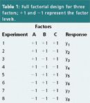
An experimental design can be considered as a series of experiments that, in general, are defined a priori and allow the influence of a predefined number of factors in a predefined number of experiments to be evaluated. For example, the table of experiments for a design that allows the evaluation of the influence of three factors (and their interactions) on the response(s) is shown in Table 1, whereas Figure 1 shows the geometric representation of the experiments.

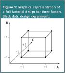
Figure 1

In Figure 2, a schematic diagram of a general experimental design-based methodology to optimize a (separation) method is shown. In the first step, when one has very little knowledge on the influence of possible factors of the technique on the responses, all factors potentially influencing the results of the method will be selected. Their effects will be evaluated in a screening step. For this purpose a so-called screening design is applied. Its aim is to identify those factors that have the largest influence on the responses of interest.

When the most important factors are selected, or when they were a priori known, their optimal combination, resulting in the best response or the best compromise between different responses, is determined. This can be done either by a simplex approach, which is a sequential procedure, or a response surface design approach. These terms will be explained in more detail later on in this article. Usually only two or three factors are studied.

When optimal conditions are selected from the above, the developed method is subjected to a validation procedure in case it will be used for quantitative purposes.

Figure 2

Towards the end of the method development or in the beginning of method validation a robustness test can be performed. This test, where an experimental design approach is also applied, was discussed in a previous column.¹ The designs used are identical to those usually executed in the screening step of method development.

Screening Designs

The purpose of these designs is to identify the important variables. The factors are evaluated at two levels. As was mentioned earlier, the designs applied are identical to those applied in robustness testing, that is, fractional factorial designs and Plackett–Burman designs.² They are two-level designs, which allow screening a relatively high number of factors in a rather low number of experiments. An example of each is given in Table 2. The different steps to be performed are also identical as in robustness testing.¹ The difference is situated in the intervals between the two levels of the factors.

Table 2(a)

In method optimization, the largest interval feasible for a given factor is considered. In robustness testing the interval is much smaller and does not exceed the experimental error much. For instance, if mobile phase pH is considered, in the first situation the levels could be, for example, 3 and 9, while a typical range in robustness testing would be optimal level ± 0.2, for example, 3.8–4.2. During execution of the design experiments a number of responses is determined and the effects of the examined factors on them are evaluated.

Figure 3

An effect of a given factor is calculated as the difference between the average results obtained when this factor was either at the low or at the high extreme levels (Table 2).¹ Frequently, the importance of the effects (i.e., their significant difference from the experimental error) is either statistically or graphically evaluated to select the most influential.¹

Simplex Approach

In the simplex approach the analyst is approaching the optimum in a sequential procedure.³ First a simplex, which is a geometrical figure defined by a number of points equal to the number of variables plus one, is executed in the experimental domain. For two variables the figure is a triangle and for three a tetrahedron. Figure?3 illustrates a situation in which a simplex approach is applied.

Figure 4

The triangles represent the simplexes and the numbers at their vertices represent the consecutive experiments. The dotted lines represent the hypothetical contour plot (unknown to the analyst) for the response to be optimized. Specific rules are applied to determine the consecutive experiments.

It can be seen that the different simplexes are moving into the direction of the optimum (here: the highest response) and finally circulate around it. The speed (the number of required experiments) and accuracy (closeness) with which the optimum is approached depend on the size of the triangles. When they are small it might take a considerable number of experiments to approach the optimum. When the simplexes are large one moves fast into the direction of the optimum but risks not being able to come close to the optimum because of the size of the simplex. To avoid that the optimum is missed because of the simplex size, variable-size simplex approaches have been developed that contain additional rules, which deal with adapting the size of the simplexes.

Response Surface Designs

The aim of these designs is to model the responses and to find the optimal combination of conditions.⁴ In these designs the factors (usually only two or three) are examined at more than two levels. The reason is that in the models, curvature of the response as a function of the factor levels is included, which requires testing of (at least) three levels.

Table 2(b)

The differences with the simplex approach are that models for the responses are built and that one assumes that the optimum of the method is situated in the experimental domain created by the selected extreme levels of the different factors.

Table 3

The most frequently applied design in this context is the central composite design (CCD). It requires nine experiments for two factors and 15 for three factors (Table 3, Figure 4). Each factor is evaluated at five levels. Other regularly applied response surface designs are three-level factorial designs, Doehlert designs and Box-Behnken designs. They will not be discussed in detail but all create a symmetric domain as for the CCD in Figure 4, when plotting the required experiments. These designs are applied when the experimental domain to examine is also symmetric or regular. Sometimes this is not the situation. An example is given in Figure 5. Such domain might be found when the organic modifier content and the pH of the aqueous fraction in the mobile phase are optimized.

Figure 5

For example, at a given pH the organic modifier content can be limited between given intervals caused by an excessively high or absent retention of the substances to be separated. When these limits are different for different pH values an asymmetric domain is obtained. Now when one wants to fit a symmetric design, such as a Doehlert design [the hexagonal shapes in Figure 5(a)], either a large part of the domain will not be examined or a number of impossible experiments will be required, depending on the factor-level range selected. The first would occur when applying design a–g; the second for design 1–7 (experiments 3,4,7 outside the feasible domain). To overcome this problem asymmetric designs are applied. Examples are the D-optimal design, and the Kennard and Stone algorithm. The idea is that in the domain a grid of potentially executable experiments [circles in Figure 5(b)] is drawn/defined.

Figure 6

The above designs then select a number of experiments, which are well distributed over the domain [for instance, full dots in Figure 5(b)]. This selection is based on different criteria. For the D-optimal design: from all possible selections of a given number of experiments (a number that is specified a priori and depends on the model built) that for which the determinant of the product of the design matrix X with its transposal X^T, det(X^T *X), is maximal is chosen. In the Kennard and Stone algorithm the experiments are selected sequentially. The first two are those for which the Euclidian distance⁴ among all possible selections is largest. The third is the experiment for which the minimal Euclidian distance to the previous selected points is largest etc.

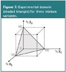
Figure 7

The model built from the response surface design results is usually the general linear model, which looks, for two factors, as

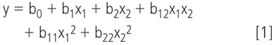
where y is a response considered (e.g., retention time/factor, peak width), x₁ and x₂ the factors considered (e.g., organic modifier content, mobile phase pH), and b_i the regression coefficients of the model. Often such a model is visually represented as a response surface (Figure 6). From model and/or surface plot, the optimal conditions are derived.

A special instance is mixture variables (e.g., the mobile phase solvents). They are not all independent (i.e., in a mixture with m compounds only m–1 can be defined independently). The fact that factor levels can be set independent from the levels of other factors is a requirement in all the above mentioned designs. Therefore, when included in such a design only m–1 mixture compounds can be examined as independent factors, while the m^th is the adjusting compound to bring the mixture to unity. For example, in a mobile phase containing water and methanol, only fractions of one solvent can be evaluated.

When only mixture variables are examined, mixture designs are applied. Because of the above restriction the experimental domain formed by mixture variables is specific. For instance, for three variables it is triangular (Figure 7); for four tetrahedral. Mixture designs are designs where the experiments are situated on the vertices, sides and/or within those specific domains. They allow modelling and constructing response surfaces. A special application of a mixture design in chromatography is the use of the solvent triangle to optimize the organic modifier composition of a mobile phase.⁵

In an optimization procedure several responses should often be optimized. The optimal conditions for one response are not necessarily those for another. Often one has a kind of conflicting situation. For instance, let us consider resolution and analysis time as responses. The first is to be maximized, the latter to be minimized. Conditions leading to a higher resolution usually will also lead to a longer analysis time and vice versa (Figure 6). Therefore, a suitable compromise between both responses needs to be found. This is possible using so-called multicriteria decision-making methods. Examples of the latter are overlays of contour plots of the response surfaces, the Pareto optimality approach and the desirability functions of Derringer.⁴

This article gave a short overview of experimental design approaches in method development and optimization. Several items, including the handling of the results, design construction, design properties, differences between designs to examine a given number of factors, simplex approach rules, domain restrictions in mixture designs, could only be touched superficially. These will be discussed in more detail in future articles.

Yvan Vander Heyden is a professor at the Vrije Universiteit Brussel, Belgium, department of analytical chemistry and pharmaceutical technology, and heads a research group on chemometrics and separation science.

References

1. B. Dejaegher and Y. Vander Heyden, LCGC Eur.,19(7), 418–423 (2006).

2. Y. Vander Heyden et al., J. Pharm. Biomed. Anal., 24(5–6), 723–753 (2001).

3. Y. Vander Heyden et al., Optimization strategies for HPLC and CZE, in K. Valko (Ed.), Handbook of Analytical Separations: Volume 1, Separation Methods in Drug Synthesis and Purification, Elsevier, Amsterdam (2000) pp. 163–212.

4. D.L. Massart et al., Handbook of Chemometrics and Qualimetrics : Part A, Elsevier, Amsterdam, 1997.

5. J.L. Glajch et al., J. Chromatogr.,199, 57–79 (1980).