Gradient Elution, Part III: Surprises

Sometimes when changes are made to gradient conditions, the result isn't what was expected.

This is the third installment in a series of "LC Troubleshooting" columns about gradient elution. Hopefully, if we can gain a better understanding about how gradients work, we'll be able to better address gradient liquid chromatography (LC) problems when they occur, or better yet, avoid them in the first place. In the first installment (1), we looked at how intuitive reversed-phase isocratic separations are, and learned some ways to transfer this intuition about the separation to gradient conditions. In the last column (2), we were introduced to the concept of the gradient retention factor, k*, and saw how it was analogous to the isocratic retention factor, k. With sufficient care, we were able to transfer our knowledge of isocratic behavior to gradient conditions. This month, we'll continue the discussion, but we'll focus on some of the surprises that can occur when the same changes are made to isocratic and gradient methods. We'll be looking at what are sometimes referred to as the "column conditions," that is, changes in column size, packing particle size, and flow rate. And to remind you, there is much more detail on this and other related gradient topics in reference 3.

Changes in Isocratic Conditions

Let's follow our pattern of looking at an isocratic example first, because usually the chromatogram changes in a predictable manner when we make a change in the column conditions. Figure 1 contains five simulated chromatograms that illustrate what happens when we make specific changes. In Figure 1a, the inset shows the reference conditions that are used. In all the chromatograms, the first small peak is the disturbance at the column dead time, t₀; the remaining eight peaks are eluted in the same order. I marked some of the peaks to make it easier to follow the discussion. In each of the other chromatograms, the inset shows one or more variables in bold type that have been changed relative to the reference case. For example, in Figure 1b, the flow rate has been changed from 2 mL/min in the reference case to 1 mL/min. Let's next look at each of the changes illustrated in Figure 1.

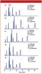
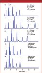
Figure 1: Simulated chromatograms for the isocratic separation of phthalic acid, 2-nitrobenzoic acid, 4-chloroaniline, 2-fluorobenzoic acid, 3-nitrobenzoic acid, 3-fluorobenzoic acid, 2,6-dimethylbenzoic acid, and 2-chloroaniline (in order of retention times): (a) reference conditions, (b) change in flow rate, (c) change in column length, (d) change in column inner diameter and flow rate, (e) change in packing particle size. The changes in each case are shown in bold in the summary of conditions. Adapted from reference 4.

A reduction in the flow rate is expected to double the retention time, and this is seen in Figure 1b; the column back pressure also should drop by a factor of two (not shown). There is a minor improvement in the resolution of peaks 2 and 3, as seen by a slightly deeper valley between the peaks. This is because the column plate number, N, increases slightly at lower flow rates, but this is rarely of much advantage with modern 3- and 5-µm particle columns when used with real samples. A change in column length from 100 mm to 150 mm in Figure 1c also has the expected result. When all other factors are held constant, we expect the retention time and the pressure to change by the ratio of the length change, or 150/100, and this is what we see. We also see a small improvement in resolution of peaks 2 and 3. Remember that N is proportional to the column length and resolution is proportional to the square root of the plate number. So resolution would be expected to improve by (150/100)^0.5 = 22%, a benefit that we achieve at the cost of a longer run and higher pressure.

Sometimes it is beneficial to reduce the column inner diameter, d_c, to save solvent, sharpen peaks, or improve compatibility with an evaporative detector such as a mass spectrometer, an evaporative light-scattering detector, or a charged aerosol detector. When the diameter is reduced, there may be an excessive increase in the back pressure if no other changes are made, so it is customary to reduce the flow rate so that the linear velocity of the mobile phase stays the same and retention times are unchanged. So when the column diameter is reduced, the flow rate should be reduced in proportion to the change in the cross-sectional area. For the reduction in column diameter from 4.6 mm to 2.1 mm shown in Figure 1d, the column cross-sectional area changes by (4.6/2.1)² , or approximately fivefold. So we reduce the flow rate from 2 mL/min to 0.4 mL/min and expect to see the same retention times and separation as in the reference case. This can be seen by comparing the chromatograms of Figures 1a and 1d.

The final change in Figure 1 is to increase the packing particle size, d_p, from 3 µm to 5 µm. This is expected to reduce N in proportion to the change, 5/3. It also should reduce resolution by the square root of this ratio, (5/3)^0.5 ≈ 1.3; this can be seen by the noticeable loss in resolution between peaks 2 and 3 in Figure 1e. The back pressure should change with the square of the particle size change, so we would expect the pressure to drop by (5/3)² , or to approximately 35% of its original value (not shown). The particle size should have no influence on retention or peak spacing if the same particle chemistry is used (same brand of packing material).

Corresponding Gradient Changes

There wasn't anything surprising about the results when we changed column conditions for an isocratic separation. Our intuition and experience helped us know what to expect. Let's see if the same expectations can be achieved when similar changes are made to a gradient separation. In Figure 2, I've chosen gradient conditions for the same sample that give approximately the same separation, as can be seen by comparing Figure 1a with Figure 2a. The peak spacing and critical resolution between peaks 2 and 3 is quite similar.

Figure 2: Simulated chromatograms for the gradient separation of the same sample as in Figure 1. (a)–(d) Same changes as in Figure 1, (e) change in flow rate and gradient time.

The reference chromatogram for the gradient separation (Figure 2a) uses a linear gradient of 20–45% B in 5 min; as with Figure 1, changes made to the conditions for the remaining chromatograms of Figure 1 are shown in bold in the inset summaries. First, let's change the flow rate from 2 mL/min to 1 mL/min in Figure 2b. We expect the retention times to double and a minor increase in resolution as we saw in Figure 1b. But this isn't what we observe. The retention times increase, but by less than a factor of two. The resolution between peaks 2 and 3 increases much more than we expected, but peak 3 now runs into peak 4. Things are not going according to our expectations.

In Figure 2c, we see the results of increasing the column length from 100 mm to 150 mm, which should increase the plate number, resolution, and run time. Here again, we see that the expected increase in retention by 50% hasn't occurred; we observe a smaller increase. And although the separation of peaks 2 and 3 increased, as we expected, we did not expect that the resolution of peaks 3 and 4 would be compromised.

Figure 2d shows the results for the reduction in column diameter with a simultaneous change in flow rate to keep the linear velocity constant. This should have no effect on the separation, and this is what we observe. The minor increase in retention can be attributed to the fact that we reduced the flow rate by a factor of 5.0, when the true ratio should be 4.8. In a similar manner, our expectations are met when we increase the particle size from 3 µm to 5 µm in Figure 2e. You can see the slight loss in resolution by examining the separation of peaks 2 and 3. At least something behaves as expected with gradients.

What's Going On?

As is probably apparent by now, there are some fundamental differences between isocratic and gradient separations that account for the differences in behavior between the two techniques when the column conditions are changed. In particular, we're interested in changes in peak spacing, expressed as the selectivity, α:

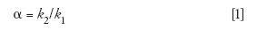
where k₁ and k₂ are the k-values for two adjacent peaks. Whenever a variable is changed in an LC separation that changes k for one or both peaks of a peak pair, a change in α will occur. The exception is when k₁ and k₂ change in proportion, but this is the exception rather than the rule with most samples under reversed-phase conditions.

Recall that the isocratic k value is calculated as

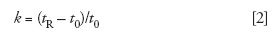
where t_R is the retention time and t₀ is the column dead time. A change in column dimensions or flow rate will change both t_R and t₀ by the same proportion, so k will stay the same, and no change in α will occur. A longer column, lower flow rate, and smaller particles each will increase the column plate number, so resolution will improve because of this, not because the peaks move relative to each other.

The gradient retention factor, k*, is calculated in a different manner than isocratic k:

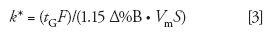
where t_G is the gradient time (in minutes), F is the flow rate (in milliliters per minute), Δ%B is the gradient range (5–95% B = 0.9), V_m is the column volume (in milliliters), and S is a constant for a given compound. Recall from last month's discussion (2) that k* is approximately the same for all peaks in a gradient separation. However, because S varies from one compound to another, small differences in k* will be seen for the various peaks in a separation; this is useful, because it allows us to make changes in some chromatographic variables so that we can optimize a gradient separation. For the current discussion, we're only concerned with changes in the column conditions — length, diameter, flow rate, and particle size — so we can simplify equation 3 to

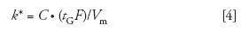
where C is a constant.

Now let's consider each of the changes to the column conditions we made in Figures 1 and 2 in light of equation 4 to see if we can make sense of the unexpected changes in Figure 2. When the flow rate was reduced from 2 mL/min to 1 mL/min in Figure 2b, we see from equation 4 that the k* value also dropped by a factor of two. This, in turn, results in a change in α (equation 1) for at least some of the peak pairs. This accounts for the increase in the separation between peaks 2 and 3 and reduction of the resolution between peaks 3 and 4; it also looks like the separation between the last two peaks has increased. The reduced flow rate increased the run time, but because k* is smaller, the run time did not double like it did in Figure 1b for the isocratic case.

An increase in the column length from 100 mm to 150 mm is shown in Figure 2c. Again consulting equation 4, we see that because V_m is directly proportional to column length, it will reduce k* by 100/150. This change in k* has a similar change in α as does the reduction in flow rate, but because the change is by less than a factor of two, peak 3 and 4 are not so closely merged in Figure 2c as they are in Figure 2b. The increase in column length does give the expected increase in N, but the predicted increase in retention by 150/100 is compromised by the reduction in k*.

For the experiment of Figure 2d, we reduced the column diameter from 4.6 mm to 2.1 mm, but we also reduced the flow rate from 2 mL/min to 0.4 mL/min to keep the mobile-phase velocity the same. The chromatogram is almost identical as the original run of Figure 2a, with a slight change in retention that we explained earlier. When we consider equation 4, we can see that the ratio of F/V_m is almost identical in the two cases: 2/4.6² ≈ 0.4/2.1² , so k* stays constant, as does α and resolution.

The final change in Figure 2e was to change the particle size from 3 µm to 5 µm. Note that the particle size, d_m, does not appear in equation 3, so it should have no influence on k*. Its only effect is to reduce the plate number and reduce pressure in the same fashion as it does in the isocratic case.

In the example of Figure 2d, we simultaneously changed the column diameter and the flow rate to keep the linear velocity constant, but this also had the effect of keeping k* constant. This is a key concept: whenever a change is made in the column conditions, a compensating change in another part of the column conditions must be made to keep k* constant or we will risk a change in α, which may be detrimental to the separation. This compensating change also is illustrated in Figure 2e. In this case, the same change in flow rate was made as was made in Figure 2b, from 2 mL/min to 1 mL/min, but in addition, the gradient time, t_G, was increased by twofold so that k* would stay constant. Thus, the peak spacing didn't change. The run time doubled, and the resolution increased marginally because the lower flow rate gave a slight increase in the plate number.

Summary

When we made changes in the column conditions (length, diameter, particle size, or flow rate) under isocratic conditions, the observed chromatograms matched our expectations. However, when we made the same changes in a gradient separation, sometimes the results were quite surprising. Isocratic k values (equation 2) are not influenced by changes in the column conditions, so peak spacing, α (equation 1) won't change, either. This is not the case with gradients, because k* is influenced by the flow rate and the column volume (equation 3), so when changes in these factors are made, a change in k* results, with a corresponding change in α. We found that if we made compensating adjustments, using equation 4 for a guide, we could change the column conditions for a gradient separation and get the expected result. The key learning point here is if changes in the column conditions are made for a gradient separation, compensating changes must be made to keep k* constant, or the separation is likely to undergo undesirable changes.

References

(1) J.W. Dolan, LCGC North Amer. 31(3), 204–209 (2013).

(2) J.W. Dolan, LCGC North Amer. 31(4), 300–305 (2013).

(3) L.R. Snyder, J.J. Kirkland, and J.W. Dolan, Introduction to Modern Liquid Chromatography, 3rd Ed. (Wiley, Hoboken, New Jersey, 2010).

(4) P.L. Zhu, L.R. Snyder, J.W. Dolan, N.M. Djordjevic, D.W. Hill, L.C. Sander, and T.J. Waeghe, J. Chromatogr. A 756, 21–39 (1996).

John W. Dolan

John W. Dolan "LC Troubleshooting" Editor John Dolan has been writing "LC Troubleshooting" for LCGC for more than 25 years. One of the industry's most respected professionals, John is currently the Vice President of and a principal instructor for LC Resources, Walnut Creek, California. He is also a member of LCGC's editorial advisory board. Direct correspondence about this column via e-mail to John.Dolan@LCResources.com