An Open-Source Simulator for Exploring HPLC Theory

Despite the utility of high performance liquid chromatography (HPLC) simulators, we found that all the free and low-cost simulators were outdated or had extremely limited functionality, so we created one that addressed these shortcomings. We developed a sophisticated, open-source HPLC simulator that is available for free as well as a version for Android users called "HPLC Simulator." Here we discuss a few questions that the simulator can help answer: Why are peaks narrower in gradient elution? What is gradient delay and how does it affect a separation? How much does extracolumn tubing affect a separation?

It is quite challenging to gain a deep understanding of the fundamental relationships that govern high performance liquid chromatography (HPLC) separations, especially gradient separations because there are a large number of strongly coupled experimental factors that affect them. For example, a seemingly simple change to just one experimental parameter - say, the flow rate - not only affects the length of a run, but also the gradient delay, back pressure, resolution of the separation, relative band spacing (that is, the selectivity), column dead time, time required to return to the initial solvent composition between runs, and separation efficiency. HPLC theory is well-developed; equations describe all of the important relationships, but there are an intimidating number of them and the dependencies between some are quite complex.

HPLC simulators provide a way to quickly gain a more intuitive understanding of the complex relationships between operating variables (1–3). They let you test a host of experimental parameters and instantly see their effect on the resulting chromatogram. Simulators can also let you try out different experimental conditions before you set up the wrong experiment or buy the wrong column, and they are useful in the laboratory when you want to calculate parameters like the back pressure or peak width that should be expected under a certain set of conditions.

Despite their utility, we found that all the free and low-cost simulators were outdated or had extremely limited functionality (4–6), so we created one that addressed these shortcomings. We developed a sophisticated, open-source HPLC simulator that is available for free at www.hplcsimulator.org (7) as well as a version for Android users called "HPLC Simulator." This simulator has controls and indicators for a wide range of experimental parameters (Table I) and displays simulated chromatograms (Figure 1). The web site also hosts another type of simulator called "HPLC Fluid Visualizer," which allows HPLC system parts such as valves and columns to be dropped onto a virtual workspace and connected with tubing to simulate the different valve configurations before they are built.

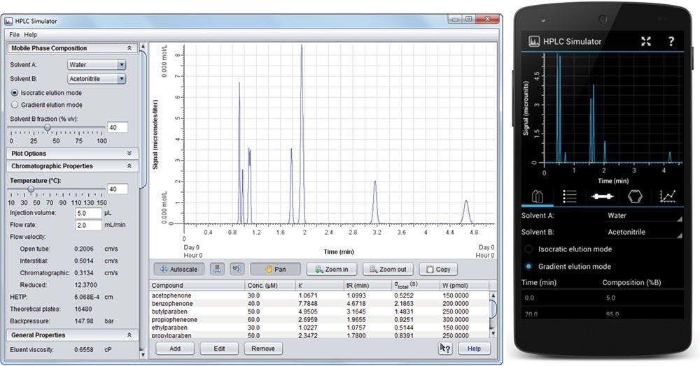
Figure 1: HPLC Simulator interface for the on-line version (left) and the mobile app (right).

We find that even experienced chromatographers can learn something by working with the HPLC simulator. The simulator can help answer a number of questions that aren't obvious to most.

Why Are Peaks Narrower in Gradient Elution?

One advantage of an HPLC simulator over a real system is that it allows you to see what's going on inside the column. Figure 2 shows plots of the position of p-xylene in the column as a function of time under isocratic and gradient elution (gray line). In isocratic elution, the compound moves through the entire length of the column at the same rate, but in gradient elution, it accelerates as the mobile phase becomes stronger. At the time the compound exits the column in gradient elution, it is moving significantly faster than when it exits the column under isocratic conditions. Therefore, the main reason peaks are relatively narrow in gradient elution is that, at the time they exit the column, they are moving faster, causing the entire band to exit the column in a shorter period of time (8). On the other hand, peaks generally exit the column more slowly under isocratic elution, spreading them out over time.

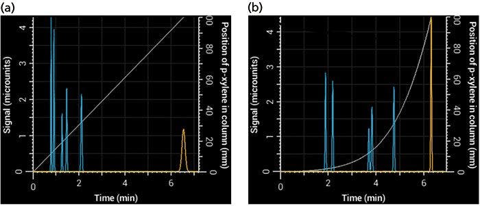
Figure 2: Simulated chromatograms obtained using (a) isocratic and (b) gradient elution. The p-xylene peak is shown in yellow, and the light gray relationship, which relates to the right-most y-axis, shows its position in the column as a function of time. At the point where p-xylene exits the column, it is moving much faster in gradient elution than in isocratic elution (the slope of the gray line is steeper), giving rise to a narrower peak (σ = 1.1 s in gradient elution versus 4.1 s in isocratic elution) even though conditions were selected that gave them the same retention times.

What Is Gradient Delay and How Does It Affect a Separation?

No HPLC system can produce a perfect gradient. At the very least, every HPLC system shows two imperfections: gradient delay, which is the delay from the time a gradient begins to be produced in the pump to when it actually reaches the column inlet, and gradient dispersion, which is the rounding of the gradient (this is the fluidic equivalent of what happens to a voltage time ramp as it passes through a low pass resistor–capacitor [RC] filter). This is a serious problem when transferring methods between instruments - the same nominal gradient yields different peak patterns (9).

To see what effect these parameters have on a separation, you can adjust the simulated pump's nonmixing volume (responsible for delay) and mixing volume (responsible for dispersion and delay). After adjusting these two parameters, you will see the resulting gradient produced by the pump and how it affects the resulting separation. Figure 3 shows a simulated separation using a 1-mm i.d. column that adequately separated acetophenone when the mixing volume was very small, but yielded a poor separation with a large mixing volume.

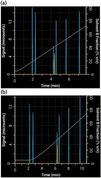
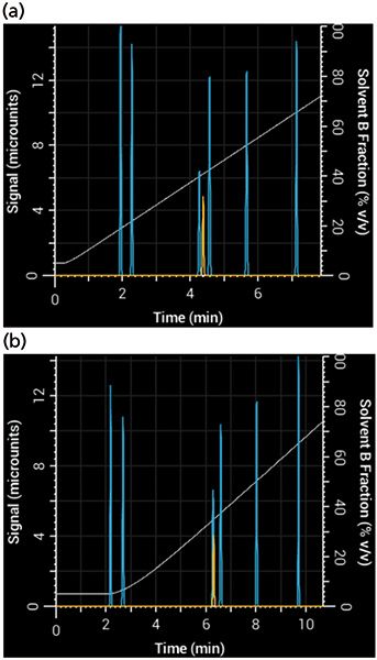
Figure 3: Effects of gradient delay and dispersion in a 10-min gradient from 5% to 95% B: Simulated separation of acetophenone (yellow) (a) using a system with very small mixing and nonmixing volumes (20 µL each) and (b) the same gradient, run on a system with larger mixing and nonmixing volumes (100 µL and 200 µL, respectively).

How Much Does Extracolumn Tubing Affect a Separation?

Postcolumn tubing can be easy to overlook, but under some circumstances it is a major contributor to band broadening. The broadening is a result of Aris-Taylor dispersion within the tube (10), which increases with increases in tubing length, tubing internal diameter, and flow rate. It becomes especially important when using columns of a small internal diameter, where the volume occupied by each band is relatively small - any broadening in the tubing causes a big increase in peak width. For example, consider a column of 1 mm i.d. with a 1.8-µm particle size, run at a flow rate of 100 µL/min using a 5-min 5–95% gradient. If 75 cm of 0.005-in. i.d. tubing were added between the column and the detector, that addition would almost double the total peak width. Figure 4 shows a simulated separation of acetophenone and 3-phenyl propanol on a 1-mm i.d. column with and without the postcolumn tubing.

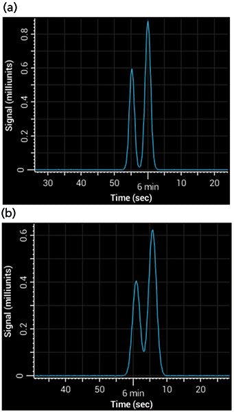
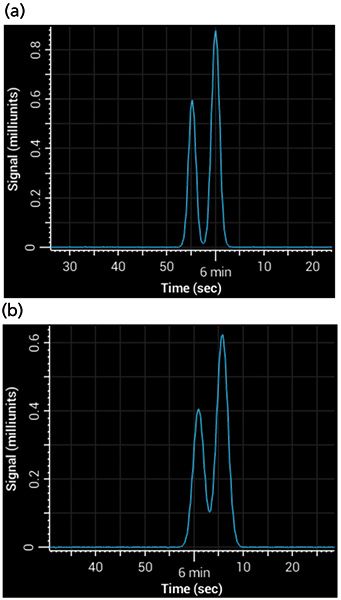
Figure 4: Simulated separations showing the effects of band broadening from postcolumn tubing: (a) Gradient separation of acetophenone and 3-phenyl propanol with near baseline resolution, simulating no postcolumn tubing; (b) separation under same conditions, but using 75 cm of 0.005-in. i.d. tubing.

Is My Injection Volume Appropriate for My Isocratic Separation?

Injection volume is less of an issue during gradient elution because well-retained compounds focus at the inlet of the column during the beginning of the gradient, effectively mitigating precolumn sources of peak broadening. However, in isocratic separations, injection volumes that are too large can cause significant additional broadening in peaks - this effect is referred to as volume overload, which is different from peak broadening that results from mass overload (8). Injecting more sample increases signal intensity, but over-injection leads to significant peak broadening. This effect can be seen in Figure 5, where too large of an injection volume resulted in broader peaks and poor resolution. The signal of phenol (1.2 min) is barely above noise in the left panel (Figure 5a), but a fivefold increase in injection volume to increase signal led to significant broadening and loss of resolution (Figure 5b). A good rule of thumb is that the injection volume will not affect peak widths significantly if it is kept below 5% of the total column volume (calculated as an open tube and assuming that the solvent composition of the sample and eluent are the same).

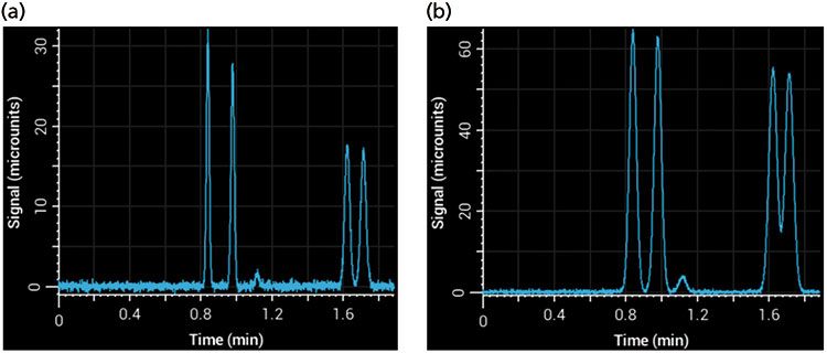
Figure 5: Simulated separations showing the effects of injection volume on an isocratic separation using a 100 mm × 2.1 mm column (with a column volume of approximately 340 µL): (a) Injection volume of 5 µL; (b) injection volume of 25 µL.

Acetonitrile Versus Methanol - Does It Make Much of a Difference?

The Snyder polarity index of water is 9, while those of acetonitrile and methanol are 6.2 and 6.6, respectively. It might seem, then, that the two solvents are nearly interchangeable. Not so! The selectivity of a separation can change considerably depending on which one you use (8). Figure 6 shows a simulated separation with acetonitrile as organic modifier and the same separation with methanol, with a resulting overall broadening of the peaks and loss of resolution between the compounds. Notice the change in selectivity between the two mobile phases - phenol (peak 3) and 3-phenyl propanol (peak 4) switch elution order depending on which one is used. Back pressure is also affected strongly by the change of organic modifier. Figure 6 also shows the simulated back pressure as a function of time during the gradient for each separation. Methanol–water mixtures have significantly higher viscosity than acetonitrile–water mixtures, producing considerably higher back pressures.

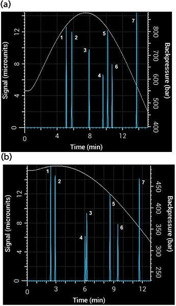
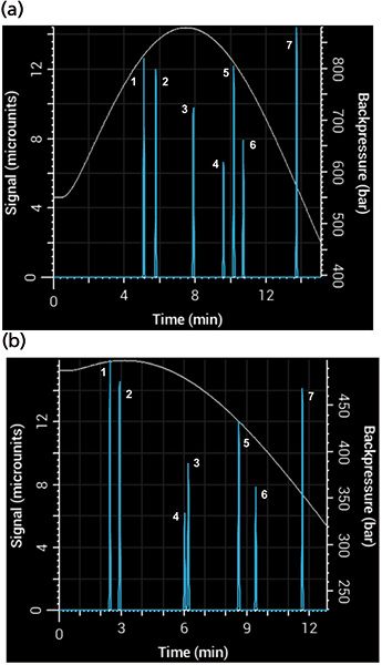
Figure 6: Simulated separations showing differences in back pressure and selectivity using (a) methanol and (b) acetonitrile mobile phase in a 5-min gradient from 5% to 95% B using a 100 mm × 2.1 mm, 3.5-µm column.

How Does Gradient Steepness Affect Peak Spacing?

One of the easiest and most efficient ways to change the selectivity of a gradient separation is to modify its steepness. Changing the gradient steepness is analogous to changing the solvent composition in isocratic separations in terms of both retention and selectivity. To understand why, consider that in a linear gradient, each compound's retention time is dependent on its "gradient steepness parameter," b, which is defined by equation 1 (11):

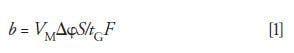
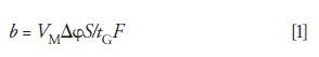
where V_M is the column dead volume, ΔΦ is the change in mobile phase composition, t_G is the gradient time, F is the flow rate, and S is a compound-specific property that represents the slope of its log k versus mobile-phase composition (Φ) relationship. Because the S parameter is compound-dependent, a change to any one of the other parameters in equation 1 (V_M, ΔΦ, t_G, or F) causes an unequal change to each compound's b parameter, which causes a disproportionate change in their retention times. Unless each compound's gradient steepness parameter is held constant, the selectivity of the separation changes.

Changing the gradient slope is the most intuitive way to change the gradient steepness, but it is not the only way to change it. Equation 1 shows that the gradient steepness can also be changed by adjusting the flow rate or column dimensions. Take, for example, the 10-component separation shown in Figure 7 using a 30-min linear gradient at 2 mL/min and a 50 mm × 4.6 mm column (Figure 7a), which resulted in multiple coeluted peaks (1 and 2 as well as 7 and 8). If V_M is increased by using a 150 mm × 4.6 mm column and t_G is decreased to 10 min, then b increases ninefold and the selectivity changes substantially (Figure 7b). In this separation there were no coeluted peaks, and the order of elution changed for several peaks as well.

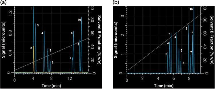
Figure 7: Differences in band spacing because of changes in gradient steepness parameter b between two gradients: Simulated separations obtained with (a) an initial 30-min gradient using a 50 mm × 4.6 mm column, and (b) with t_G decreased to 10 min and column length increased to 150 mm.

How Can a Method Be Changed Without Altering Selectivity (or Resolution)?

The previous section showed that the selectivity of a separation can be altered by changing the gradient steepness, but sometimes the goal is rather to change one or more method parameters (for example, particle size, column dimensions, or gradient time) while maintaining the same selectivity and sometimes also the same resolution. This process is also known as method translation (12).

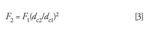
To keep selectivity constant, the gradient steepness must be kept constant; if a parameter from equation 1 changes, then it must be offset by a change to another parameter in the equation. To keep resolution constant as well, then the number of theoretical plates, N, must also be held constant. The number of theoretical plates is directly proportional to the column length and inversely proportional to the particle size, so to keep N constant, the following relationship must be true:

where L₁ and L₂ are the lengths of the original and new columns, and d_p1 and d_p2 are the particle size of the original and new columns, respectively. The number of theoretical plates is also dependent on the flow velocity, but the relationship is less predictable (a van Deemter relationship), so the flow velocity is often left unchanged to ensure the same resolution.

Let's consider an instance where we want to translate a linear 20-min, 2-mL/min gradient that used an old 150 mm × 4.6 mm column with 5-µm particles to a newer 2.1-mm i.d. column with 1.8-µm particles. Using equation 2 we find that the new column length must be approximately 50 mm. To keep the same linear velocity, we can calculate the new flow rate by using equation 3:

where F₁ and F₂ are the flow rate of the original and new method, and d_c1 and d_c2 are the internal diameter of the original and new columns, respectively. Based on our choice of using a 2.1-mm i.d. column, the new flow rate is approximately 0.42 mL/min. Finally, we can use equation 1 to find the new gradient time, t_G2, that is required to keep b constant with the new values of V_M and F, thus keeping the selectivity constant. This results in a new gradient time of approximately 6.5 min. Figure 8 shows our initial separation translated to a shorter separation using our new column dimensions and particle size while keeping the same selectivity and resolution. Note that in this example we used a simulated system with no gradient delay volume, but an important caveat to keeping the same selectivity (particularly of early eluted compounds) is that the ratio between gradient delay volume and column dead volume must be kept constant (9).

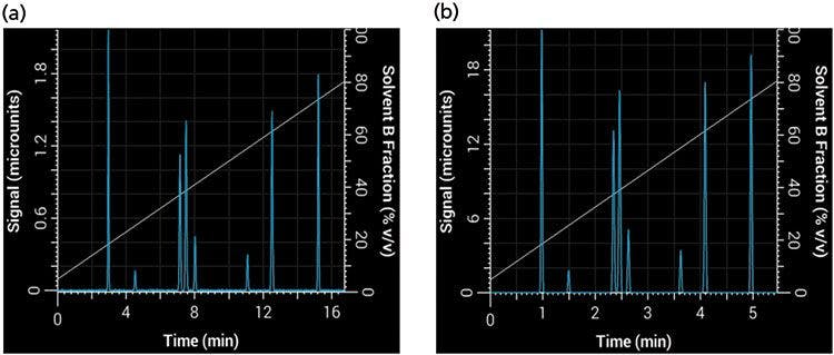
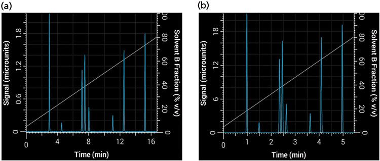
Figure 8: Translation of a linear gradient to a shorter gradient time and column while keeping the same selectivity and resolution: Simulated separations obtained using (a) the original linear 20-min, 2-mL/min method with a 150 mm × 4.6 mm, 5-µm column; (b) a 6.5-min, 0.42-mL/min method with a 50 mm × 2.1 mm, 1.8-µm column.

Conclusion

In addition to these topics, the HPLC simulator can also be used to demonstrate more-basic concepts such as the general elution problem or the dependence of retention on solvent composition and temperature. Is there anything else you'd like modeled? We are always looking for ways to improve the simulator. Send us a message via e-mail and we'll try to put it in a future release.

Acknowledgments

We thank the National Institute of General Medical Sciences of the National Institutes of Health [R01GM098290] for supporting this project. We also thank Jonathan E. Turner, Bonnie A. Alden, and Michael P. Balogh at Waters for helping measure retention data for the Waters stationary phase in the simulator.

References

(1) R.C. Rittenhouse, J. Chem. Educ. 65, 1050–1051 (1988).

(2) D.C. Stone, J. Chem. Educ. 84, 1488–1496 (2007).

(3) I.C. Bowater and I.G. McWilliam, J. Chem. Educ. 71, 674–678 (1994).

(4) J.C. Reijenga, J. Chromatogr. A 903, 41–48 (2000).

(5) R.A. Shalliker, S. Kayillo, and G.R. Dennis, J. Chem. Educ. 85, 1265–1268 (2008).

(6) R.C. Rittenhouse, J. Chem. Educ. 72, 1086–1087 (1995).

(7) P.G. Boswell, D.R. Stoll, P.W. Carr, M.L. Nagel, M.F. Vitha, and G.A. Mabbott, J. Chem. Educ. 90, 198–202 (2013).

(8) L.R. Snyder, J.J. Kirkland, and J.W. Dolan, Introduction to Modern Liquid Chromatography, 3rd Ed. (John Wiley & Sons, Hoboken, New Jersey, 2010), pp. 405–497.

(9) A.P. Schellinger and P.W. Carr, J. Chromatogr. A 1077, 110–119 (2005).

(10) G. Taylor, Proc. R. Soc. London A. 219, 186–203 (1953).

(11) J.W. Dolan and L.R. Snyder, J. Chromatogr. A 799, 21–34 (1998).

(12) D. Guillarme, J.-L. Veuthey, and V. Meyer, LCGC Eur. 21, 322–327 (2008).

Daniel Abate-Pella and Paul G. Boswell are with the Department of Horticultural Science at the University of Minnesota in St. Paul, Minnesota. Dwight R. Stoll is with the Department of Chemistry at Gustavus Adolphus College in St. Peter, Minnesota. Peter W. Carr is with the Department of Chemistry at the University of Minnesota in Minneapolis, Minnesota. Direct correspondence to: bosw0011@umn.edu