Quantification of Individual Mass Transfer Phenomena in Liquid Chromatography for Further Improvement of Column Efficiency

This article reports on the physical phenomena that control column efficiency and on experimental protocols designed to accurately measure their contributions to band broadening of analytes during their passage from the injection to the detection device. The results of these protocols are analyzed, allowing for the accurate determination of the complete mass transfer mechanism in different separation modes and providing solutions and future directions to further improve the efficiency of liquid chromatography columns.  

The successful separation of complex mixtures and critical pairs of similar compounds by liquid chromatography (LC) ultimately depends on how many plates the chromatographic column can generate. This need for higher plate numbers has continuously pushed column manufacturers forward to produce finer particles from about 100 μm in the early days of LC (1,2) down to nearly 1 μm today thanks to the advent of ultrahigh-pressure liquid chromatography (UHPLC) in the mid-2000s (3,4). From a practical viewpoint, LC practitioners often wonder what causes their peak widths to become unexpectedly large under certain experimental conditions and, therefore, they search for some rationale or, at least, reasonable explanations for their observations. The scientific principles and theories of band broadening and mass transfer in LC columns have continuously been revisited over the last 50 years. They were recently reviewed, refined, and adjusted based on the accumulation of a large amount of accurate experimental data and validated computer-simulated data (5). The lack of and need for a quantitative measurement of the different physical phenomena involved in the overall band broadening of a sample molecule as it progresses from the injection loop through the column and to the detection cell unit were addressed. The combination of a series of experimental protocols necessary to unravel the complete mass transfer mechanism in a chromatographic column was then proposed (6).

In the 1960s, Giddings established the most general and comprehensive theory of band broadening in chromatographic columns (7). It is still valid today. The finite width of an eluted peak results from the combination of several independent sources of sample dispersion. They include longitudinal diffusion (the B/u term in the van Deemter equation), eddy dispersion caused by mobile-phase velocity inequalities (the A(u) term), and solid–liquid mass transfer resistance due to the finite rate of diffusion across the stationary phase and to slow adsorption–desorption (the Cu term). To those three main height equivalent to a theoretical plate (HETP) terms, one can add extracolumn band broadening, which has become increasingly important with the new generation of sub-2-μm particles and narrow-bore columns operated in UHPLC (8,9), and the friction of the mobile phase against the packed bed (generating heat) and its expansion during the inlet-to-outlet decompression (consuming heat), which both cause additional peak band broadening under nonadiabatic conditions (5).

The first purpose of this work is to redefine all the potential sources of band broadening inside and outside the chromatographic column and to discuss when, in practice, each of them is dominant in LC. The second goal is to illustrate how the B/u, A(u), and Cu HETP terms of the van Deemter equation can be accurately measured from a series of well designed protocols. These quantitative results are used to decipher the complete mass transfer mechanism in reversed-phase LC C18 columns packed with 2.5-μm fully porous particles and 2.6-μm superficially porous particles, in hydrophilic interaction chromatography (HILIC) columns packed with 3.5-μm fully porous particles, in chiral reversed-phase columns packed with 5-μm fully porous particles coated with cellulose polymer, and in reversed-phase LC C18 silica-based monolithic columns of the first and second generation. The final goal is to reveal from these experimental investigations the key directions to follow for the improvement of the efficiency of the future generation of LC columns.

Column Efficiency: A Dimensionless Approach

The efficiency of a chromatographic column, which is defined as the ratio of its length (L) to its plate height (H), is a function of a very large number of physical parameters. These are the linear velocity of the mobile phase (u, cm/s), the particle size or the characteristic size of the separation medium (d_p, cm), the diffusion coefficient of the analyte in the bulk mobile phase (D_m, cm²/s), the diffusivity of the analyte in the stationary phase (D_p = Ω D_m, cm²/s), the retention factor (k'), the external porosity of the chromatographic bed (ε_e), the bed aspect ratio or the ratio of the inner diameter of the column to the particle size (d_c/d_p), and the ratio of the column length to its diameter (L/d_c). A simpler, easy-to-use relationship between the column efficiency N and these experimental variables is needed. This can be achieved from a dimensionless approach that is familiar in chemical engineering (7). The column efficiency N is first normalized to the column length (plate height) and to the particle size to define the reduced plate height (h):

The linear velocity u is reduced to the particle diameter and the bulk diffusion coefficient of the analyte. This defines the reduced velocity (ν) as

These two dimensionless variables are related through a general expression, the dimensionless or reduced van Deemter equation (10):

The kinetic performance of the column is now a function of only three variables (B, A, and C), which vary little provided that the practitioner operates with a certain retention mode (such as HILIC, reversed-phase LC, chiral LC, or ion-exchange chromatography) and uses a similar column format (short or wide internal diameter columns, capillary columns, particulate, or monolithic columns). B accounts for the longitudinal diffusion along the packed bed immersed in the eluent; A accounts for all sources of eddies in the column; and C accounts for the finite rate of diffusion across the stationary phase and the potentially slow adsorption–desorption process.

The advantage of equation 3 is straightforward: Chromatographers can easily anticipate, with a good approximation, the efficiency of any given column under various experimental conditions. For instance, the left graph in Figure 1 illustrates the expected change in the reduced plate height h when transferring a method from high performance liquid chromatography (HPLC) to UHPLC (large to small particle size, low to high pressures). For the maximum allowable pressure (400 bar in HPLC and 1200 bar in UHPLC), the reduced velocities are smaller in UHPLC than those in HPLC because of the diminution of both the particle size (× 1/3) and the linear velocity (the column permeability decreases by about one order of magnitude because it is proportional to the square of the particle diameter). Therefore, at maximum pressure, the column efficiency of UHPLC columns is essentially controlled by the longitudinal diffusion B/ν and the eddy dispersion A(ν) HETP terms in the van Deemter equation, and in conventional HPLC the column efficiency is governed by the A(ν) and Cν HETP terms. The right graph in Figure 1 shows the shifts in reduced velocity and plate height when using the same column, but for different applications (small to large molecules, same linear velocity). When analyzing large biomolecules (~10 kDa) instead of small molecules (<500 Da), the bulk diffusion coefficient typically decreases by one order of magnitude. The reduced velocity increases then by a factor of 10 and the column efficiency essentially becomes dependent on the slow rate of diffusion across the stationary phase: it is mostly controlled by the Cν HETP term.

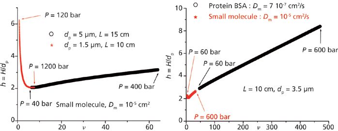
Figure 1: Impact of the experimental chromatographic conditions (conventional HPLC versus UHPLC, left graph; analysis of small and large molecules, right graph) on the expected reduced plate height and column efficiency. The universal reduced van Deemter plot (B, A, and C coefficients) was obtained for a conventional 150 mm × 4.6 mm C18 reversed-phase LC column and a retention factor of about 3.

The Different Sources of Band Broadening in LC

The different physical phenomena causing the chromatographic band to broaden are redefined and listed below.

Extracolumn Band Broadening

Band broadening does not only take place inside the column. To some extent, the chromatographic system itself also contributes to sample dispersion after the passage of the injected sample volume along the injection loop, the needle seat capillary (in most HPLC instruments), the injection valve, the inlet and outlet capillaries, and the detection cell (including its electronic components [11]). About 15 years ago, analysts did not have to worry much about extracolumn band broadening in LC because the column dimensions were large enough and the column efficiency still moderate when 250 mm × 4.6 mm and 5 μm were the standard column format and particle size, respectively. Indeed, the volume variance of the chromatographic peak because of the sole chromatographic column is given by equation 4(8):

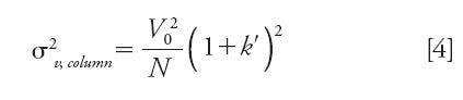
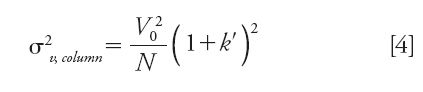
According to equation 4, the system contribution to the total peak variance observed by the analyst becomes increasingly important when small diameter columns (small hold-up volume V₀) are packed with fine particles (large efficiency N) or when small retention factors k' are applied. In 2014, with the emergence of sub-2-μm core–shell particles packed in 100 mm × 2.1 mm columns, the intrinsic efficiencies of LC columns can now reach values close to 450,000 plates/m (d_p = 1.3 μm [4]). Unfortunately, this exceptionally high level of efficiency cannot be achieved or observed by analysts because of the band broadening along the UHPLC instrument, even with the most advanced instruments. Figure 2 illustrates this statement by plotting the maximum system volume variance required to observe at least a certain fraction (p) of the maximum intrinsic plate number (d_p = 1.6 μm, core-shell particles, N_intrinsic = 39,000 for a 100 mm × 2.1 mm column) versus the retention factor k'. For instance, if a chromatographer imposes p = 90%, this goal (N_observed = 0.9 × 39,000 = 35,100) can only be satisfied with system 1, system 2, or system 3 if k' is larger than 8, 5, and 2, respectively. If p = 50%, the k' values should only be larger than about 2 and 1 for systems 1 and 2, while the goal set for N_observed = 0.5 × 39,000 = 19,500 will always be satisfied with system 3 irrespective of the retention factor. The importance of instrumentation for fast liquid chromatography in pharmaceutical applications was recently documented (69).

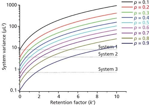
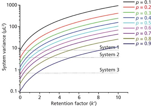
Figure 2: Plot of the minimum system variance versus the retention factor k' required to observe at least a certain fraction p of the maximum intrinsic plate number (N_max = 39,000 plates for a 100 mm × 2.1 mm column packed with 1.6-mm core–shell particles).

Longitudinal Diffusion

Longitudinal diffusion is caused by the inescapable relaxation of the axial concentration gradients during the residence time of the sample zone in the chromatographic column. More quantitatively, this source of band broadening is directly dependent on the effective diffusion coefficient (D_eff) of the analyte along the heterogeneous bed made of a solid porous material, the internal eluent (its average composition may differ from that of the bulk mobile phase), and the external mobile phase. The coefficient B in the reduced van Deemter equation is given by equation 5 (5):

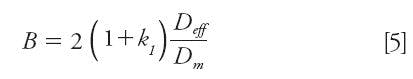
where k₁ is the zone retention factor.

Longitudinal diffusion is dominant for low reduced velocities (small linear velocity u, large diffusion coefficient D_m, and small particle diameter d_p) and is dependent on the sample diffusivity inside the stationary phase (d_p = Ω D_m), which affects the value of D_eff (12). This is particularly true in reversed-phase LC because of so-called "surface diffusion" in the stationary phase (13–15) unlike in HILIC (16) or chiral chromatography (17) where the intraparticle diffusivity is the smallest and is mostly controlled by the sole pore diffusion (18).

Solid–Liquid Mass Transfer Resistance Because of a Finite Rate of Diffusion Across the Stationary Phase

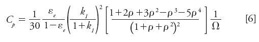
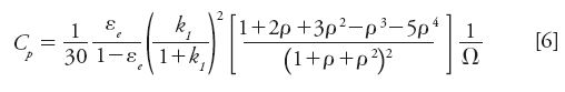
This source of band dispersion is because of the velocity difference between molecules trapped inside the stationary phase (zero velocity) and those of other molecules, which simultaneously progress forward along the column in the interstitial mobile phase at an average linear velocity (u). Assuming spherical particles and a radial symmetry for the diffusion process across the porous particles, the general expression of the reduced mass transfer coefficient (C_ρ) for core–shell particles (ρ is the core-to-particle diameter ratio; ρ = 0 for fully porous particles) is given by (19):

The contribution of the solid–liquid mass transfer resistance to the overall peak width is important for the largest reduced velocities (ν) (fast average linear velocity u, large particle diameter d_p, small diffusion coefficient D_m), the lowest reduced intraparticle diffusivities (Ω), and the largest zone retention factors k₁.

Eddy Dispersion

Band broadening because of eddy dispersion is related to all sources of velocity biases in the interstitial eluent. Additionally, these velocity biases combine with the border effects associated with the nonideal distribution and collection of the sample zone at the inlet and outlet of the column, respectively. Eddy dispersion is divided into two categories: the short range and the long range (7).

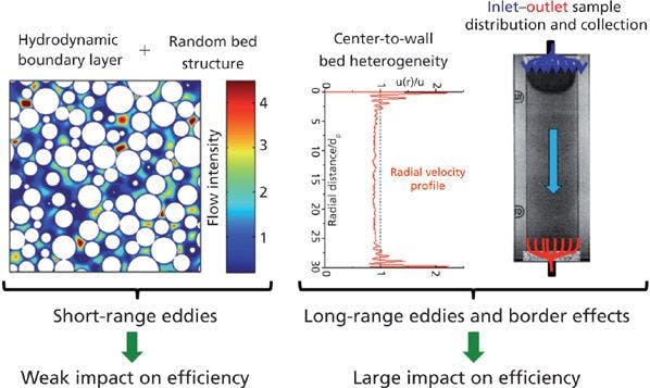
Figure 3: Visualization of short-range and long-range eddy dispersion in a packed column. Adapted with permission from reference 67.

Short-Range Eddy Dispersion

Short-range eddy dispersion involves all the velocity biases that take place over distances smaller than a few particle diameters. The left graph in Figure 3 shows the square cross-section area of the bulk region of a packed bed (the particles are represented in white) with the intensity (from dark blue for the lowest local velocities to brown for the largest ones) of the local eluent velocity along the direction normal to this surface. Significant differences in fluid velocity are observed between those at the surface of the particle (zero velocity, dark blue) and those in the center of the interstitial volumes between adjacent particles (maximum velocity, brown). This represents the so-called transchannel eddy dispersion (7). Smaller differences in the mobile phase velocity are also observed over distances covering one to a few particle diameters because of the random structure of a packed bed. This accounts for the so-called short-range interchannel eddy dispersion (7). These two HETP terms are additive and each is quantitatively described by the Giddings's coupling theory of eddy dispersion. Their sum is written as follows (7):

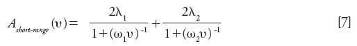
The two pairs of parameters λ₁ and ω₁ (trans-channel eddy dispersion) and λ₂ and ω₂ (short-range interchannel eddy dispersion) can either be guessed (as Giddings did in his book on dynamics of chromatography [7]) or measured from the reconstruction of the actual three-dimensional (3D) bulk structures of packed beds (with nonporous particles) after numerically solving the Navier-Stokes equations for the determination of the complete flow field u(x,y,z) along these bulk structures and calculating the band dispersion (H) from a standard advection-diffusion model. Examples are available in the literature for columns packed with core–shell particles (20) and for silica-based monolithic columns (21). They permit the correction and adjustment of Giddings's original guesses for the four parameters in equation 7. In real columns, the impact of the short-range eddy dispersion on column efficiency is small compared to that of the long-range eddy dispersion, which is defined in the next section.

Long-Range Eddy Dispersion

The presence of a cylindrical wall surrounding the packed bed (the stainless steel column tube) induces a radial heterogeneity of the bed structure across the column diameter. This is illustrated in the central plot of Figure 3 for a 50-μm i.d. capillary column packed with 1.7-μm particles. A peripheral and a central region can be clearly distinguished. The thickness of the wall region is about five times the particle size (d_p). The average interstitial velocity in this peripheral volume is close to 10% larger than the average velocity in the bulk central region of the capillary column. This long-range eddy dispersion (also called transcolumn eddy dispersion [7]) is combined with the nonidealities of the distribution and collection of the sample zone at the inlet and outlet of the column, respectively. The right graph in Figure 3 shows that the sample molecules do not actually enter the packed bed as a perfectly flat rectangular plug, but rather as a bowl (see the trajectories along the blue lines). Regarding the sample collection through the central aperture of the outlet endfitting, it takes a slightly longer time for a molecule located in the wall and corner region of the column to be eluted than for those present in its central zone. This is illustrated by the red streamlines in the right graph of Figure 3. The long-range eddy dispersion accounts for at least 50% and up to 90% of the total plate height of small molecules at high reduced velocities (5).

Adsorption–Desorption Kinetics

When the number of adsorption–desorption steps (from the internal eluent to the surface of the mesopores for adsorption and vice versa for desorption) during the migration of the analyte along the column becomes too small, both the plate height and the peak skewness (asymmetry) can reach excessively large values. This result was predicted a long time ago by the molecular or stochastic theory of chromatography (2), and it is usually observed for large molecules involving slow conformational changes in the stationary phase (27) and in chiral chromatography (17). The number of adsorption steps is governed by the rate constant of adsorption k_ads (unit Hz), which depends on four independent properties of the adsorption system, as shown in equation 8 and explained below:

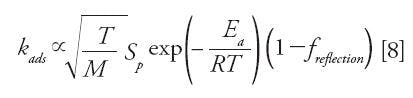
• k_ads is proportional to the average molecular speed of the analyte in the bulk phase in contact with the solid adsorbent.

• High temperatures and low-molecular-weight compounds contribute to increase the number of adsorption steps. It is also proportional to the specific surface area per volume unit of the adsorbent (S_p).

• Porous particles with a larger surface-to-volume ratio are preferred. However, the adsorption process is also characterized by the activation energy for adsorption because only a fraction of the analytes with an energy equal to or larger than E_a can be adsorbed. Again, high temperatures are definitely recommended to increase the intensity of k_ads.

• Finally, even though some analyte molecules have the required energy for adsorption (E > E_a), a fraction of them (f_reflection) will not be adsorbed because they simply bounce back to the internal eluent after collision with the solid adsorbent. Therefore, this stresses the importance and need for a high surface coverage of the bonded ligand in chiral separations.

Assuming a first-order adsorption–desorption kinetics (Langmuir adsorption), the contribution (C_ads) of the adsorption–desorption process to the overall coefficient C = C_p + C_ads in the reduced van Deemter equation 3 is given by equation 9 (28):

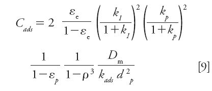
where k_p is the retention factor for the particle volume only (no external eluent) (28).

Recent investigations have shown that when k_ads is larger than 104 Hz, the adsorption–desorption kinetics has no impact on the column efficiency and on the peak resolution in LC (29). That is the case for most reversed-phase LC and HILIC applications based on the analysis of small molecules. This is no longer the case in chiral chromatography for the analysis of large biomolecules.

Friction Expansion of the Mobile Phase

Under certain operating conditions, such as high pressures in UHPLC, large linear velocities in HPLC, an external thermal environment with a thermostated column wall, nonadiabatic thermal conditions in general, and expansible eluents used in supercritical fluid chromatography (SFC), the friction of the mobile phase against the packed bed and its decompression can be accompanied by either a significant production (when friction dominates) or adsorption (when decompression dominates) of heat in the packed bed volume. Overall, the heat power generated per unit length of the column is given by equation 10 (22):

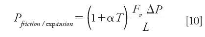
where α (<0) is the thermal expansion coefficient of the eluent, T is the temperature, F_v is the flow rate, and ΔP is the pressure drop along the column.

In UHPLC, the average product αT is around –1/3 (23) (1 + αT is positive) so that a significant amount of heat can be produced inside the column for the largest product of the flow rate by the pressure drop. A first fraction of this heat is dissipated out of the column by convection (at the column outlet) and by conduction (at the column wall). The remaining fraction is dissipated by conduction, which produces radial temperature gradients and, therefore, radial gradients of the local migration velocity for retained compounds across the column diameter. The intensity of this fraction depends on the thermal environment of the column (adiabatic versus nonadiabatic). It usually represents about 25% of the heat produced by friction when the column is kept horizontal under still-air conditions (68). Severe band distortions are then observed, as shown in the left graph of Figure 4 when the wall temperature is uniformly maintained (24). Analyte molecules in the hot central region of the column migrate faster than those in the cooler wall region. Inversely, in SFC the pressure drops are relatively small but the product of the thermal expansion of pure carbon dioxide by the temperature is around –10 (25) (1 + αT is negative). Heat is now absorbed by the column and the temperature at the center of the column is cooler than the temperature of its peripheral region. Overall, the effect on column efficiency is the same as in UHPLC and the peak shape becomes severely affected (see Figure 4b).

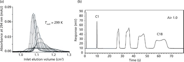
Figure 4: Visualization of peak distortion in (a) UHPLC and (b) SFC. Adapted with permission from references 21 and 22.

Measurement of the Various Sources of Band Broadening in LC

In this section, a series of experimental protocols are proposed for the experimental determination of the reduced longitudinal coefficient (B) (12,30), including: the solid–liquid mass transfer resistance coefficient (C_p) because of finite diffusion across the stationary phase (5,6), the short-range (31) and long-range eddy dispersion A(ν) terms (6), and the solid–liquid mass transfer resistance coefficient (C_ads) because of the slow adsorption–desorption process (17). Before performing these measurements, the diffusion coefficient of the analyte in the bulk phase should first be accurately measured.

The Bulk Diffusion Coefficient D_m

All of the effective diffusion coefficients involved in the chromatographic process (such as the effective diffusivity [D_eff] along the heterogeneous packed bed made of particles immersed in the liquid phase and the intraparticle diffusivity [D_p]) are scaled to the bulk diffusion coefficient (D_m). The measurement of D_m is also necessary for the determination of the reduced velocity (ν). Two methods are available: the peak parking method and the capillary method.

The Peak Parking Method

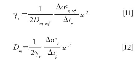
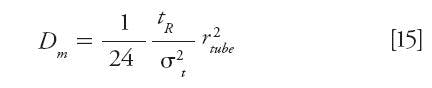
This method consists of parking the sample zone inside a column packed with nonporous particles at the very same axial position for a series of increasing arresting times (t_p) and in recording the time peak variance (σ_t²) of the eluted band (32). The best slope of the expected linear plot of σ_t² versus t_p provides an excellent estimate (within 5%) of the diffusion coefficient (D_m) as long as the analyte is not retained on the surface of the nonporous particles and that a reference standard is available for which the diffusion coefficient D_m,ref is known accurately. This reference compound permits the measurement of the external obstruction factor (γ_e) of the column used in this protocol. If u is the linear velocity applied for the elution of the sample zone, the expressions of γ_e and D_m are then directly given by equations 11 and 12 (5):

The Capillary Method

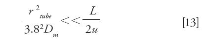
If the studied compound is adsorbed onto the nonporous particles, then the capillary method can be a suitable alternative solution (33,34). It is valid if the following five conditions are satisfied:

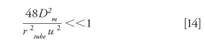
• The radial equilibration of the sample concentration is effective along a tube of length (L) and inner radius (r_tube), operated at the average linear velocity u. This condition is achieved when (35)

• The contribution of axial molecular diffusion to the total spatial variance is negligible. This condition is achieved if (36)

• The extracapillary time peak variance is negligible compared to the observed time variance.

• There is no secondary flow circulation in the coiled tube. The product of the Dean number by the Schmidt number should be smaller than 100 (37).

• The diffusion coefficient of the studied compound is validated from the value D_m,ref measured for a standard reference compound for which the true diffusion coefficient is accurately and independently known from another technique.

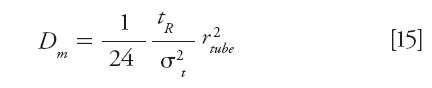
Using the capillary method, only one injection is necessary. The diffusion coefficient is then obtained from the retention time (t_R) and the time peak variance (σ_t²) of the eluted peak:

The Reduced Longitudinal Coefficient B

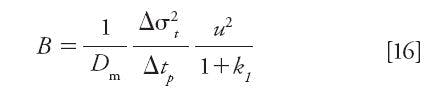
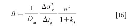
The reduced B coefficient in the reduced plate height equation is measured from the peak parking method described above using the column of interest. Figure 5 shows the typical and expected observations when increasing the peak parking time (t_p): the peak width becomes larger and the time peak variance increases linearly with increasing t_p. The most relevant experimental information includes the best slope of the linear plot shown in the Figure 5b, the zone retention factor k₁ that can be measured from a single injection for t_p = 0, and the applied constant linear velocity u during the peak parking experiments. B is then given by equation 16 (6):

The Reduced Mass Transfer Coefficient C_p

The determination of this mass transfer coefficient is relatively approximate and challenging compared to that of the coefficient B. First, it is based on the assumption that the symmetry of diffusion across the spherical particles is strictly radial (so that the concentration is uniform at the external surface area of the particles). The general expression of C_p for core–shell particles is given by equation 6 (19). Secondly, the parameter Ω or the ratio of the intraparticle diffusivity D_p to the bulk diffusion coefficient D_m in equation 6 is unknown and must be estimated. This can be done by combining the previous peak parking results for the determination of the B coefficient and the selection of a validated mathematical model of effective diffusion along the chromatographic bed (38). By simple inversion of the mathematical formula of the best model of effective diffusion, the parameter Ω can be extracted and C_p can be estimated directly from equation 6. See reference 5 for the list of available models of effective diffusion in chromatographic beds.

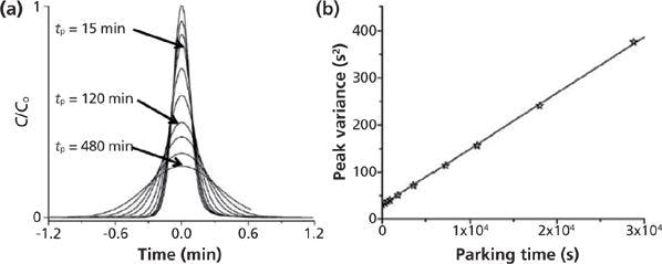
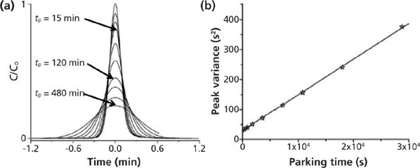
Figure 5: Illustration of the peak parking method applied for thiourea on an endcapped C1 5-μm column (150 mm × 4.6 mm) using 75:25 (v/v) methanol–water as the mobile phase. Flow rate: 0.5 mL/min. (a) Eluted peaks for different peak parking times (0, 5, 10, 15, 30, 60, 120, 180, 300, and 480 min). (b) Corresponding plot of the time peak variance versus the arresting time. Adapted with permission from reference 30.

The Reduced Short-Range Eddy Dispersion A_SR(ν)

No chromatographic methods are currently available for the direct measurement of the short-range eddy dispersion in real chromatographic columns term because columns have an inlet, an outlet, and a wall boundary. These boundaries induce an additional source of eddy dispersion (the so-called long-range eddy dispersion) as previously described and illustrated in the middle and right graphs of Figure 3. Therefore, original and different approaches were recently developed based on either a computer-based (39,40) or an image-based (41–43) reconstruction of the actual bulk random structure of packed beds. The computer-based approach is based on the Jodrey-Tory algorithm with independent adjustment of the bed porosity (from random dense to random loose packings) and degree of heterogeneity (from long-range uniform to long-range heterogeneous distribution of spherical particles). The image-based approach involves confocal laser scanning microscopy (CLSM) in combination with a sophisticated treatment of the image data (41). It has been successfully applied to the direct visualization of the homogeneous, random structure of both particulate and monolithic columns as shown in Figure 6. After the precise 3D structure of the bulk region of the chromatographic bed is known, the flow field and the band broadening of analytes along these structures can be calculated and used to measure the best coefficients λ₁, ω₁, λ₂, and ω₂ in equation 7.

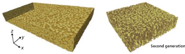
Figure 6: Visualization of the bulk, homogeneous, and random structures of packed (left) and silica-based monolithic (right) columns from confocal laser scanning microscopy and image analysis. Adapted with permission from reference 42.

The Reduced Long-Range Eddy Dispersion A_LR(ν)

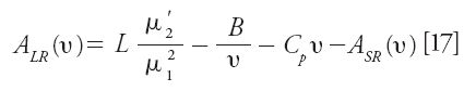
The long-range eddy dispersion HETP term, which results from the border and wall effects on band broadening in relatively short or wide columns, is accessible experimentally provided that the friction-expansion HETP term previously described can be neglected and the adsorption–desorption kinetics is fast enough (k_ads > 104 Hz). A_LR(ν) is then directly measured after subtraction of the B/ν, C_pν, and A_SR(ν) HETP terms from the total reduced HETP, h, obtained from the numerical integration of the whole peak for the determination of the first (μ₁) and second central (μ₂') moments (44):

The Apparent Adsorption Rate Constant k_ads

In a recent attempt to identify and quantify the different sources of band broadening in a cellulose-based chiral column, the adsorption rate constant (k_ads) was estimated by assuming a homogeneous adsorption process (only one adsorption rate constant will be measured) and a first-order kinetics (the analytical solution of the general rate model of chromatography is available after Laplace transform) (17). Accordingly, the expression of the corresponding reduced HETP term, C_adsν, is given by equation 9. The method was based on the use of an achiral compound and an achiral column for the estimation of the long-range eddy dispersion A_LR(ν) of the chiral column. The achiral column was not randomly picked: It should have the same dimensions (length and inner diameter) as those of the chiral column, should be packed with particles having the same size as the particles in the chiral column, and should be slurry-packed by the same column manufacturer (same column endfitting, same column tube, comparable slurry-packing process). Therefore, the long-range eddy dispersion is likely to be similar on both the chiral and achiral columns. The advantage of the achiral column is that its long-range eddy dispersion HETP can be directly measured from equation 16 since the adsorption–desorption process is fast enough and does not contribute to the total reduced HETP. This choice for the achiral column was validated from the injection of the achiral compound onto the chiral column and by comparing its total HETP to the sum of B/ν, C_pν, A_SR(ν) (all three of these HETP terms were measured on the chiral column as mentioned above), and A_LR(ν) (the only HETP term measured on the achiral column). Figure 7 compares these two reduced HETP plots for tri-tert-butylbenzene (nonchiral compound, Figure 7a) and (R,S) trans-stilbene oxide (chiral compound, Figure 7b). The observed difference between the red and black symbols represents the contribution of the adsorption–desorption kinetics HETP term to the total plate height. The term k_ads can finally be estimated from equation 9 and the best slope of the plot of this h difference versus the reduced velocity (ν).

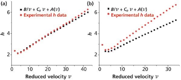
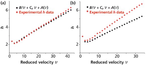
Figure 7: Comparison of the total HETP measured on a chiral column (red symbols) and the sum of the longitudinal diffusion (B/ν), the solid–liquid mass transfer resistance because of a finite diffusivity across the stationary phase (Cν), the short-range eddy dispersion (all three measured on the chiral column), and the long-range eddy dispersion (measured on a reference arbitrary achiral column). The analytes were (a) the achiral compound tri-tert-butylbenzene and (b) the chiral compound (R,S) trans-stilbene oxide. Adapted with permission from reference 17.

The Extracolumn Volume Variance σ_v,ex²

The measurement of extracolumn band broadening should be performed without replacing the chromatographic column with a zero-dead-volume union connector. Indeed, the back pressure generated by the zero-dead-volume union connector is much smaller compared to that generated by the column. Because the pressure affects the diffusion coefficients (the eluent viscosity increases with increasing pressure), it also has an impact on the sample band broadening in the precolumn volume of the instrument (45). When the extracolumn volume is much smaller than the hold-up column volume, the use of a series of homologous compounds (such as n-alkybenzenes or n-alkylphenones) allows for the noninvasive measurement of the system band broadening (46). The plot of the apparent plate height as a function of the reciprocal of (1 + k')² is expected to be linear provided that the intrinsic plate height varies little with increasing retention factor:

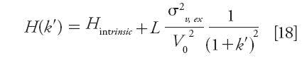
Knowing the column length (L) and the hold-up column volume (V₀), the slope of this representation provides directly the system volume variance σ_v,ex². This experimental protocol was recently applied to a series of n-alkylphenones using four different configurations of UHPLC instruments. Their extracolumn volume variance increases from about 0.5 to 3, 10, and 40 μL² (46). Figure 8 shows the corresponding plots of H versus (1 + k')^-2 for a 100 mm × 2.1 mm column packed with 1.6-μm core–shell particles at a constant flow rate of 0.4 mL/min. The experimental plots are quasilinear and their y-intercept is virtually the same and equal to the intrinsic plate height of the column. The significant difference in the observed slopes reflects directly on the different levels of band spreading along the four UHPLC systems reported in the legend of the graph.

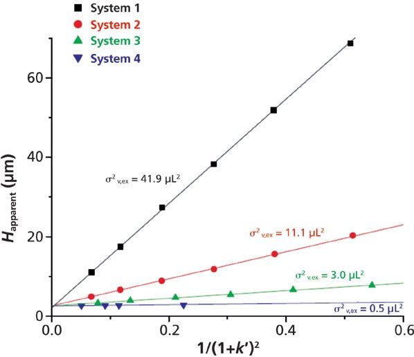
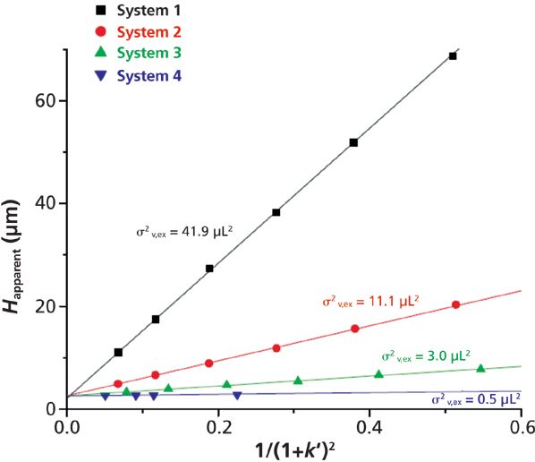
Figure 8: Plots of the apparent HETPs of homologous compounds versus the reciprocal of (1 + k')² for four different UHPLC instruments. Column: 100 mm × 2.1 mm packed with 1.6-μm prototype reversed-phase LC C18 core–shell particles. Eluent: 75:25 (v/v) acetonitrile–water. Temperature = 24 °C. Note that the system 2 has been modified with 140-μm i.d. connectors. It is not representative of the commercial standard instrument. Adapted with permission from reference 46.

Determining the Mass Transfer Mechanism in Different Columns and LC Retention Modes

The experimental protocols described in the previous sections are applied here for the determination of the complete mass transfer mechanism of four different classes of chromatographic columns: reversed-phase LC C18 columns packed with fully and superficially porous particles, reversed-phase LC C18 silica-based monolithic columns, a HILIC column packed with fully porous particles, and a cellulosed-based chiral reversed-phase column packed with fully porous particles.

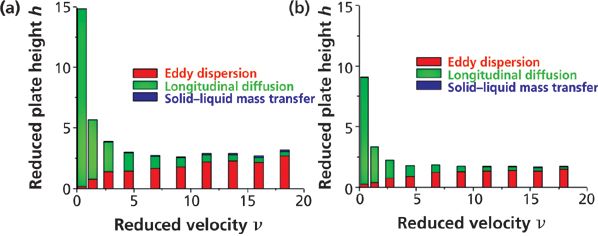
Figure 9: Contributions of the longitudinal diffusion (green), eddy dispersion (red), and solid–liquid mass transfer resistance (blue) terms to the overall reduced plate height of 100 mm × 4.6 mm columns packed with (a) 2.5-μm fully porous particles and (b) 2.6-μm core–shell particles. Analyte: naphthalene. Mobile phase: 65:35 (v/v) acetonitrile–water. Temperature = 297 K. Adapted with permission from reference 47.

Reversed-Phase LC Particulate Columns: Core–Shell Versus Fully Porous Particles

Figure 9 shows the contributions of the B/ν, A(ν), and C_pν HETP terms to the total observed h values for two columns having the same dimension (100 mm × 4.6 mm). One (Figure 9a) is packed with 2.5-μm fully porous particles and the second (Figure 9b) is packed with 2.6-μm core–shell particles (47). The most remarkable observation is that all three reduced HETP terms are smaller for core–shell particles. B is smaller because the impermeable solid core occupies about 25% of the column volume and sample diffusion is not allowed across the volume of these cores. This is an advantageous feature for the shell particles at the lowest reduced velocities and at those close to the optimum speed (ν_opt = 8–10). C_p is also smaller because the average length of the diffusion path across the core–shell particles is shorter. However, for small retained molecules like naphthalene (k' ≈ 3, D_m ≈ 1.5 × 10^-5 cm²/s) and 2.5-μm particles, the maximum reduced velocity is about 18 and the largest gain in HETP is just 0.1 h unit. So, in practice, the decrease of the C_pν HETP term is virtually negligible at optimum speed. Regarding the total eddy dispersion HETP A(ν) term, it is about 0.5 h units smaller for the shell than for the fully porous particles at high velocities. The question remains whether this is because of a diminution of the short- or the long-range eddy dispersion HETP. It is known that the particle size distribution (PSD) of core–shell particles is much tighter than that of conventional particles with a relative standard deviation (RSD) around 5% versus 15–25%. Figure 10 shows the calculated reduced HETPs along computer-based generated bulk structures of actual 1.7-μm fully porous particles (wide PSD) and 2.6-μm core–shell particles (narrow PSD) (48). The calculations were also carried out for monosize particles (RSD = 0%). The results demonstrated that the RSD of the PSD had no impact whatsoever on A_SR(ν) at a fixed bed porosity. In fact, A_SR(ν) is mostly a function of the bed porosity. Additionally, it is known experimentally that the external porosity of columns packed with core–shell particles is around 0.40 (49–51) versus only 0.36 for columns packed with conventional fully porous particles. Therefore, the short-range eddy dispersion is even larger for core–shell than for standard particles (48). In conclusion, the higher kinetic performance of the 2.6-μm core–shell particles shown in Figure 9 is because of a significant reduction of the long-range eddy dispersion HETP. This reflects the higher degree of homogeneity of the packed bed (from the center to the inner wall of the column tube) of columns packed with core–shell particles than that of columns packed with fully porous particles.

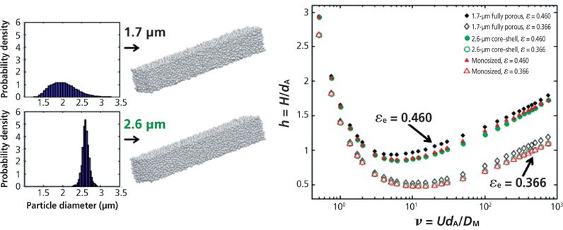
Figure 10: Effect of the RSD of the particle size distribution on the short-range eddy dispersion for dense (bed porosity = 0.366) and loose (bed porosity = 0.46) randomly packed beds. Adapted with permission from reference 48.

Reversed-Phase LC Silica-Based Monolithic Columns: First Versus Second Generation

Figure 11 shows the contribution of the same sources of band broadening as in Figure 9, but for a silica-based monolithic column (100 mm × 4.6 mm) of the first generation commercialized in the early 2000s. Remarkably, the minimum HETP is no smaller than 18 μm because of the large intensity of the eddy dispersion HETP term at and beyond the optimal velocity (52,53). The manufacturer of these monolithic columns prepared a second generation of silica-based monolithic columns (same dimension) with smaller macropore and skeleton sizes (or domain size) and a much reduced impact of the A(ν) term on the observed column efficiency (54,55). Figure 12 shows, from a quantitative viewpoint, that the total eddy dispersion HETP decreases by about 12 μm, which is considerable. The maximum column efficiency improved then from about 50,000 plates/m (for the first generation instrument) to 170,000 plates/m (for the second generation). However, the reconstruction of the bulk structures of these two types of monolithic columns and the calculation of the short-range eddy dispersion (right graph in Figure 12) revealed a difference of only 0.5 μm (54), a value far smaller than the 12 μm observed. If the silica-based monolithic columns had no wall (infinite diameter column) and no border (infinitely long column), the first and second generation of silica-based monolithic columns would generate as many as 500,000 and 625,000 plates/m. This shows evidence that the performance of 4.6-mm i.d. silica monolithic columns is controlled by either the transcolumn velocity biases or the border effects. Additionally, the analysis of the center-to-wall heterogeneity of the monolith structure by CLSM shows no significant default for the second generation column (54). In conclusion, further improvement of the efficiency of silica-based monolithic columns is linked to a better distribution and collection of the sample zone at the inlet and outlet of the column, respectively.

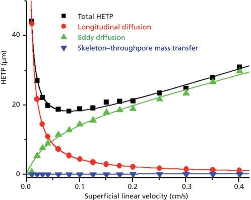
Figure 11: Contributions of the longitudinal diffusion (red), eddy dispersion (green), and solid–liquid mass transfer resistance (blue) terms to the overall reduced plate height of 100 mm × 4.6 mm silica-based reversed-phase LC monolithic column of the first generation. Analyte: naphthalene. Mobile phase: 55:45 (v/v) acetonitrile–water. Temperature = 297 K. Adapted with permission from reference 53.

Mass Transfer Mechanism in HILIC Columns

The mass transfer mechanism in HILIC columns differs from that in reversed-phase LC columns (same dimension, same particle size) because the intraparticle diffusivity is much smaller across nonbonded porous silica than across the same (but C18-bonded) silica particles. This was unambiguously revealed from the measurement of the reduced longitudinal diffusion coefficient B as shown in Figure 13 (18). For retained analytes, B is typically twice as large in reversed-phase LC as in HILIC columns because of the concentration excess of the organic eluent (acetonitrile), which forms a thick multilayer (three monolayers) onto the silica-C18 surface in reversed-phase LC (56), and the presence of a water-rich layer onto neat silica in HILIC (57). Therefore, in reversed-phase LC, the analytes are adsorbed and retained through weak dispersive interactions onto nonlocalized adsorption sites and they accumulate by a partition mechanism in a poorly viscous acetonitrile-rich eluent (the partition of the sample molecules between pure acetonitrile and the aqueous eluent is large). Their diffusion or mobility in the stationary phase is then fast. In contrast, in HILIC, the mobility of the retained analytes is relatively small because they are either strongly bound to specific adsorption sites (zero mobility) or concentrated (partition mechanism) in an aqueous layer that is three times more viscous (58,59). Consequently, the reduced coefficient C_p is larger in HILIC than in reversed-phase LC (because of the smaller intensity of the parameter Ω in equation 6 for HILIC particles) and the optimum reduced velocity is usually observed around five in HILIC instead of 10 in reversed-phase LC retention mode. This explains why reversed-phase LC has been such a successful mode of retention in LC.

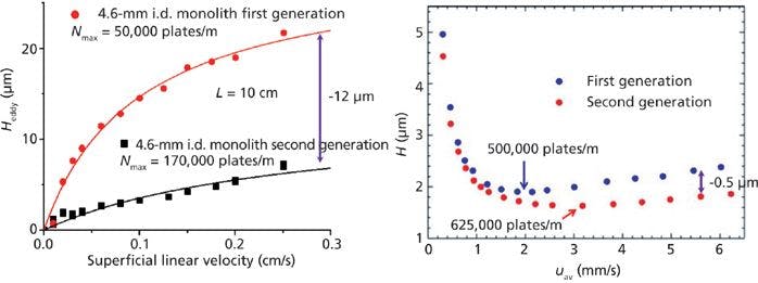
Figure 12: Diminution of the total eddy dispersion HETP (left) and comparison between the short-range eddy dispersion (right) and for the first and second generation of silica monolithic columns. Adapted with permission from references 53 and 52.

Mass Transfer Mechanism in Chiral Columns

Chiral separations may involve an additional source of band broadening compared to reversed-phase LC and HILIC retention modes. The adsorption–desorption process in chiral chromatography is usually slower than that in reversed-phase LC and HILIC columns. It can contribute significantly to the intensity of the overall C coefficient in the van Deemter plot. Figure 14 illustrates this statement by comparing the experimental reduced HETPs of reversed-phase LC C18, HILIC, and cellulosed-based chiral reversed-phase columns. The optimum reduced velocity is the smallest for the chiral reversed-phase column at about three. In the absence of activation energy (E_a) (no kinetic barrier for adsorption) and if all molecular collisions between the surface area of the adsorbent and the analyte lead to an adsorption event, then the adsorption rate constant (k_ads) would be as large as 109 Hz (60) and the adsorption–desorption process would have no impact whatsoever on column efficiency. In fact, the measurement of all the sources of band broadening in a chiral column packed with 5-μm cellulose-based particles revealed that k_ads was of the order of 103 Hz only (17). For such small values of k_ads, the kinetics of adsorption definitively limits the column performance, as shown in Figure 14. Figure 15 shows the contribution of the slow rate of adsorption–desorption to the total HETP for the enantiomer trans-stilbene oxide on a cellulose-based chiral column. Roughly, the reduced coefficient (C_ads) represents more than 50% of the total reduced coefficient C in the van Deemter plot and the band broadening because the slow adsorption rate of trans-stilbene oxide accounts for about 25% of the total plate height at a reduced velocity of 30.

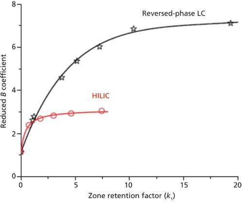
Figure 13: Comparison between the reduced longitudinal coefficient B measured on a reversed-phase LC C18 (black) and HILIC (red) column. Reproduced with permission from reference 18.

Conclusions: Further Improvement of the Observed Column Efficiency

Based on the previous experimental protocols designed for the measurement of all sources of band broadening in reversed-phase LC, HILIC, and chiral reversed-phase columns, the practitioner now has direct access to the quantitative contributions of longitudinal diffusion, eddy dispersion (short- and long-range), mass transfer resistance because of a finite rate of diffusion across the particle, mass transfer resistance because of a slow adsorption–desorption process, and of the HPLC system band spreading to the overall observed peak width. The column or instrument manufacturers are finally able to pinpoint with confidence the intrinsic weaknesses of their products. They are becoming more inclined to invest time and financial resources to cope with the relevant problems, which are limiting the column efficiency observed by their customers.

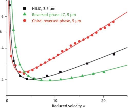
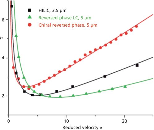
Figure 14: Comparison between the reduced longitudinal coefficients B measured on a reversed-phase LC C18 column (black) and a HILIC column (red). Reproduced with permission from reference 18.

Pursuing the transition from conventional HPLC to faster UHPLC methods, smaller column dimensions and finer particles are increasingly invading analytical laboratories. Irrespective of the retention mode applied (reversed-phase LC, HILIC, chiral), the efficiency of this new generation of chromatographic columns can be seriously limited by the band dispersion that takes place along the different parts (injection loop, valve, connecting tubes, detector, electronics) of the instrument. For instance, to get at least 80% of the intrinsic efficiency (N_intrinsic ≈ 22,500) of a 50 mm × 2.1 mm column packed with 1.3-μm core–shell particles and for a retention factor of 1 (the column volume variance is only equal to 1.6 μL²), the system band spreading should not be larger than 0.4 μL², which is a level not yet achieved even with the best UHPLC instruments currently available.

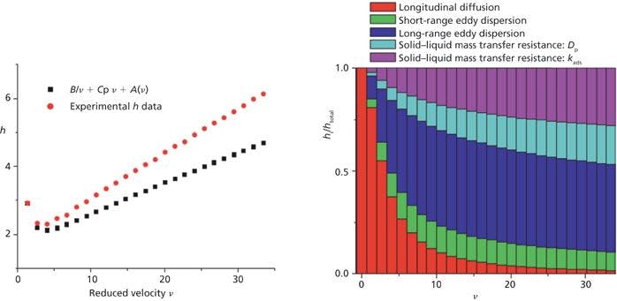
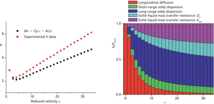
Figure 15: Impact of a slow adsorption–desorption process (k_ads) on the total reduced plate height of trans-stilbene oxide on a cellulose-based chiral stationary phase. Reproduced with permission from reference 17.

Regarding the intrinsic kinetic performance of a chromatographic column, the measurement of the eddy dispersion HETPs in reversed-phase LC, HILIC, and chiral reversed-phase columns has unambiguously revealed that it was governed by the long-range eddy dispersion. In other words, the column hardware should be redesigned to minimize the effects of the center-to-wall flow heterogeneity, of the nonideal sample distribution at the column inlet, and of the asynchronous collection of sample zone at the column outlet. Active flow technology or parallel segmented outlet (and curtain) flow chromatography was recently developed to get rid of the molecules migrating along the peripheral region of the bed (61,62). Only the molecules leaving the column through the central region of the outlet cross-section area are collected and detected. The efficiency of the shortest columns packed with sub-3-μm particles can then be multiplied by a factor close to two after elimination of the rear peak tailing and reduction of the long-range eddy dispersion (63,64). Nevertheless, it is important to remember that this new column technology also has some limitations in terms of gain in column efficiency: It is not advantageous for the longest columns (because of the radial equilibration across the whole bed diameter [64,65]), for the largest particle sizes (because of large transverse diffusion coefficients [66]), and for large molecules since the mass transfer mechanism is essentially governed by the Cν and not by the A(ν) HETP term anymore.

In conclusion, the results of this series of experimental protocols stress the need for the integration of the injection device, separation medium, and detection system into a single unit free from poor connections that can cause severe additional band broadening. Technological and scientific skills are then required in terms of miniaturization, micro- and nano-fluidics, and 3D printing to design and prepare tomorrow's most efficient separations systems (67).

References

(1) U.D. Neue, HPLC Columns, Theory, Technology, and Practice (Wiley-VCH, New York, 1997).

(2) C. Horvath, B. Preiss, and S. Lipsky, Anal. Chem.39, 1422–1428 (1967).

(3) J.R. Mazzeo, U.D. Neue, M. Kele, and R.S. Plumb, Anal. Chem. 77, 460A–467A (2005).

(4) A.C. Sanchez, G. Friedlander, S. Fekete, J. Anspach, D. Guillarme, M. Chitty, and T. Farkas, J. Chromatogr. A1311, 90–97 (2013).

(5) F. Gritti and G. Guiochon, J. Chromatogr. A1221, 2–40 (2012).

(6) F. Gritti and G. Guiochon, J. Chromatogr. A1217, 5137–5151 (2010).

(7) J.C. Giddings, Dynamics of Chromatography (Marcel Dekker, New York, 1965).

(8) F. Gritti, C. Sanchez, T. Farkas, and G. Guiochon, J. Chromatogr. A1217, 3000–3012 (2010).

(9) K.J. Fountain, U.D. Neue, E.S. Grumbach, and D.M. Diehl, J. Chromatogr. A1216, 5979–5988 (2009).

(10) J. van Deemter, F. Zuiderweg, and A. Klinkenberg, Chem. Eng. Sci.5, 271–289 (1956)

(11) J.C. Sternberg, Advances in Chromatography (Marcel Dekker, New York, 1966).

(12) F. Gritti and G. Guiochon, J. Chromatogr. A1218, 3476–3488 (2011).

(13) F. Gritti and G. Guiochon, Anal. Chem. 78, 5329–5347 (2006).

(14) K. Miyabe and G. Guiochon, J. Chromatogr. A 1217, 1713–1734 (2010).

(15) F. Gritti and G. Guiochon, AIChE J.57, 346–358 (2011).

(16) F. Gritti and G. Guiochon, J. Chromatogr. A 1302, 55–64 (2013).

(17) F. Gritti and G. Guiochon, J. Chromatogr. A1332, 35–45 (2014).

(18) F. Gritti and G. Guiochon, J. Chromatogr. A1297, 85–95 (2013).

(19) K. Kaczmarski and G. Guiochon, Anal.Chem. 79, 4648–4656 (2007).

(20) S. Bruns and U. Tallarek, J. Chromatogr. A1218, 1849–1860 (2011).

(21) K. Hormann, T. Müllner, S. Bruns, A. Höltzel, and U. Tallarek, J. Chromatogr. A1222, 46–58 (2012).

(22) H.-J. Lin and Cs. Horvath, Chem. Eng. Sci. 36, 47–55 (1981).

(23) M. Martin and G. Guiochon, J. Chromatogr. A1090, 16–38 (2005).

(24) F. Gritti and G. Guiochon, J. Chromatogr. A1216, 1353–1362 (2009).

(25) D. Poe and J. Schroden, J. Chromatogr. A1216, 7915–7926 (2009).

(26) J.C. Calvin and H. Eyring, J. Phys. Chem. 1216, 416–421 (1955).

(27) B.C.S. To and A. Lenhoff, J. Chromatogr. A1141, 191–205 (2007).

(28) K. Kaczmarski, J. Chromatogr. A1218, 951–958 (2011).

(29) F. Gritti and G. Guiochon, J. Chromatogr. A1348, 87–96 (2014).

(30) F. Gritti and G. Guiochon, Chem. Eng. Sci. 61, 7636–7650 (2006).

(31) D. Hlushkou, S. Bruns, and U. Tallarek, J. Chromatogr. A1217, 3674–3682 (2010).

(32) J.H. Knox and L. McLaren, Anal. Chem. 36, 1477–1482 (1964).

(33) J. Li and P.W. Carr, Anal. Chem.69, 2530–2536 (1997).

(34) J. Li and P.W. Carr, Anal. Chem.69, 2550–2553 (1997).

(35) G. Taylor, Proc. R. Soc. Lond. A219, 186–203 (1953).

(36) R. Aris, Proc. R. Soc. Lond. A 235, 67–77 (1956).

(37) L.A.M. Janssen, Chem. Eng. Sci.31, 215–218 (1976).

(38) F. Gritti and G. Guiochon, Chem. Eng. Sci. 66, 6168–6179 (2011).

(39) S. Khirevich, A. Höltzel, S. Ehlert, A. Seidel-Morgenstern, and U. Tallarek, Anal. Chem.81, 4937–4945 (2009).

(40) S. Khirevich, A. Höltze, A. Seidel-Morgenstern, and U. Tallarek, Anal. Chem.81, 7057–7066 (2009).

(41) S. Bruns, T. Müllner, M. Kollmann, J. Schachtner, A. Höltzel, and U. Tallarek, Anal. Chem.82, 6569–6575 (2010).

(42) D. Hlushkou, S. Bruns, A. Höltzel, and U. Tallarek, Anal. Chem.82, 7150–7159 (2010).

(43) S. Bruns, J.P. Grinias, L.E. Blue, J.W. Jorgenson, and U. Tallarek, Anal. Chem.84, 4496–4503 (2012).

(44) P. Stevenson, F. Gritti, and G. Guiochon, J. Chromatogr. A1218, 8255–8263 (2011).

(45) F. Gritti and G. Guiochon, J. Chromatogr. A (2014).

(46) F. Gritti and G. Guiochon, J. Chromatogr. A1327, 49–56 (2014).

(47) F. Gritti and G. Guiochon, LCGC North Am.30(7), 586–595 (2012).

(48) A. Daneyko, A. Höltzel, S. Khirevich, and U. Tallarek, Anal. Chem.83, 3903–3910 (2011).

(49) F. Gritti and G. Guiochon, J. Chromatogr. A1252, 31–44 (2012).

(50) F. Gritti and G. Guiochon, J. Chromatogr. A1252, 45–55 (2012).

(51) F. Gritti and G. Guiochon, J. Chromatogr. A1252, 56–66 (2012).

(52) D. Hlushkou, K. Hormann, A. Höltzel, S. Khirevich, A. Seidel-Morgenstern, and U. Tallarek, J. Chromatogr. A1303, 28–38 (2013).

(53) F. Gritti and G. Guiochon, J. Chromatogr. A1218, 5216–5227 (2011).

(54) K. Hormann and U. Tallarek, J. Chromatogr. A1312, 26–36 (2013).

(55) F. Gritti and G. Guiochon, J. Chromatogr. A1225, 79–90 (2012).

(56) F. Gritti and G. Guiochon, J. Chromatogr. A1169, 111–124 (2007).

(57) F. Gritti, A. dos Santos Pereira, P. Sandra, and G. Guiochon, J. Chromatogr. A1216, 8496–8504 (2009).

(58) S.M. Melnikov, A. Höltzel, A. Seidel-Morgenstern, and U. Tallarek, J. Phys. Chem.C 117, 6620–6631 (2013).

(59) S.M. Melnikov, A. Höltzel, A. Seidel-Morgenstern, and U. Tallarek, Anal. Chem.83, 2569–2575 (2011).

(60) D. Hlushkou, F. Gritti, A. Daneyko, G. Guiochon, and U. Tallarek, J. Phys. Chem C117, 22974–22985 (2013).

(61) M. Camenzuli, H.J. Ritchie, J.R. Ladine, and R.A. Shalliker, J. Chromatogr. A1232, 47–51 (2012).

(62) R.A. Shalliker, M. Camenzuli, L. Pereira, and H. J. Ritchie, J. Chromatogr. A1262, 64–69 (2012).

(63) F. Gritti and G. Guiochon, J. Chromatogr. A1297, 64–76 (2013).

(64) F. Gritti, J. Pynt, A. Soliven, G.R. Dennis, R.A. Shalliker, and G. Guiochon, J. Chromatogr. A1333, 32–44 (2014).

(65) A. Daneyko, D. Hlushkou, S. Khirevich, and U. Tallarek, J. Chromatogr. A1257, 98–115 (2012).

(66) A. Daneyko, D. Hlushkou, S. Khirevich, and U. Tallarek, J. Chromatogr. A1257, 98–115 (2012).

(67) F. Gritti and G. Guiochon, Anal. Chem.85, 3017–3035 (2013).

(68) F. Gritti and G. Guiochon, Anal. Chem.80, 6488–6499 (2008).

(69) S. Fekete, I. Kohler, S. Rudaz, and D. Guillarme, J. Pharm. Biomed. Anal.87, 105–119 (2014).

Fabrice Gritti is with the Department of Chemistry at the University of Tennessee in Knoxville, Tennessee. Direct correspondence to: gritti@ion.chem.utk.edu

In Memoriam

This article was written in memory of Georges Andre Guiochon, Distinguished Professor at the University of Tennessee Knoxville from 1987 to 2014. Prof. Guiochon was born on September 6, 1931, in Nantes, France, and passed away on October 21, 2014, succumbing to an old enemy, neuromuscular failure due to post-polio syndrome. He was an exceptional and dedicated scientist in separation science for nearly six decades and received numerous international Awards for his immense contributions to the field. Beyond his professional achievements and leadership, his human qualities were no less remarkable. From the early ages of gas chromatography in the 1950s to the latest developments in supercritical fluid and liquid chromatography today, he was the mentor, the charming companion, and the loyal friend of several generations of scientists all over the world. In the names of all whose lives and professional careers have been directly or indirectly influenced by Georges' wisdom and advice, I would like to offer to his whole family our deepest sympathy. Georges will be missed and his memory will live in us forever.