The Rise and Fall of Expertise in Gas Chromatography
LCGC North America

Guest columnist Walter Jennings reflects on the early days of capillary gas chromatography (GC) and how chromatographers become experts in the technology by constructing their own columns, thereby achieving a more thorough understanding of the chromatographic process.
Walter Jennings
Prof. Walter Jennings, one of the pioneers of gas chromatography, was a 2005 corecipient of the California Separation Society (CaSSS) Award for Distinguished Contributions to Separation Sciences. This column is a condensed version of his award lecture. Prof. Jennings reflects on the early days of capillary gas chromatography (GC) and how chromatographers became experts in the technology by constructing their own columns, thereby achieving a more thorough understanding of the chromatographic processes. With the advent of modern columns and sophisticated instruments to run them, some of this expertise has disappeared, especially in view of the fact that GC has become an easy-to-use routine tool for nonanalytical chemists. In his teaching on the subject, he relates how students are awakened when challenged to understand the underlying principles.
Most authorities would agree that gas chromatography (GC) is still one of the world's most widely used analytical techniques. Unfortunately, a large percentage of those currently using GC have a limited comprehension of its basic principles. The erosion of GC expertise is probably best explained by contrasting GC's early history with current conditions.
GC was first envisioned by A.J.P. Martin in 1948 and demonstrated by James and Martin in 1952. It began to enjoy wider usage in 1953 and onward. All of these early efforts employed packed columns, in which the resistance to gas flow limits practical column lengths and the total numbers of attainable theoretical plates. Golay's invention of the open tubular column alleviated this latter restriction, but claims to the contrary not withstanding, the patents on open tubular columns were rigorously enforced. In addition, the quality of the wall-coated open tubular (WCOT) columns available from the patent holder left much to be desired. Some have suggested that this might have been a factor in the patent holders apparently abrupt diversion into support-coated open tubular (SCOT) columns rather than striving to improve the quality of their WCOTs. Most early WCOT users made their own columns, ostensibly for personal use. The complications they faced included the roughness of the inner surface of the tubing, which challenges the deposition of a thin uniform film, as well as the high cost of stainless steel capillary tubing. Desty's elegantly simple machine for drawing long lengths of coiled glass capillary tubing provided a more inert tubing with a smoother inner surface that was also less expensive and introduced the age of glass capillary GC. A number of laboratories — largely in Europe and the United Kingdom, and less widely in South Africa and the United States — were soon engaged in drawing and coating glass capillary columns. Many of these were at universities and government-sponsored laboratories, but a few industrial laboratories (for example, Shell in the Netherlands, Shell, BP, and several other petroleum labs in England, Ciba Geigy in Basel, and Dow in Midland, Michigan) plus a number of individual scientists were contributing members of these elite "centers of excellence." Some authorities have argued that the rigorous patent enforcement actions retarded the development of GC (1), but it is the author's feeling that the overall effect was an unintended blessing. A large number of scientists who would have preferred to continue in their individual research efforts, but needed better columns, began instead to draw and coat glass capillary columns to further their efforts in a variety of research areas. Many of these efforts evolved into studies on improvements in coating methodologies, surface deactivation, methods and hardware for sample preparation, sample injection and detection, interfacing columns to injectors and detectors, and a wide variety of applications. Workers at these sites became thoroughly grounded in the basic principles of GC, and several centers offered educational courses in GC (for example, Rudolph Kaiser's institute at Bad Duerkheim, Germany, and later, Patrick Sandra's at Kortrijk, Belgium).
Most instrument companies lagged behind these developments — early users drastically altered commercial instruments, or constructed their own. Carlo Erba (Milan) was the earliest company to offer chromatographs that were designed for glass capillary columns. The vast majority of our columns were of mediocre quality by today's standards, with at least one notable exception: Professor Kurt Grob, whose laboratory in Duebendorf (a suburb of Zurich), Switzerland, was producing superior glass capillary columns. One of his associates, Hansjuerg Jaeggi, explored the possibilities of commercializing column production, and only by exploiting a unique provision in Swiss law were Jaeggi and Grob able to force the issuance of a license from Perkin Elmer. (There is no connection between the old Perkin Elmer and the PerkinElmer of today; they are entirely different companies.) Jaeggi's columns were so obviously superior that Perkin Elmer then approached Jaeggi with a proposal to share technology, but Perkin Elmer had made the struggle so acrimonious that Jaeggi wanted nothing more to do with them. Jaeggi produced superb columns, and much of his output was quickly purchased by the Swiss flavor and fragrance giants Firmenich (Geneva) and Givaudan (Zurich), and Kaffee Hag (Germany).
Kurt Grob then began offering courses in column manufacture, first in Europe, then in the United States. He carefully screened applicants to exclude those that might have commercial ambitions. It is my belief that he taught these courses so that budding capillary gas chromatographers had the hands-on experience of making and testing columns — it was an educational exercise ensuring that each participant had at least a minimum level of GC expertise. It seems probable that he dreaded the day when untrained individuals simply could buy a GC system, install a column, and produce chromatograms.
During the last 20 years, most of the previously mentioned "centers of excellence" have disappeared, or had their activities greatly curtailed. Universities have failed to replace retiring faculty whose efforts in analytical chemistry contributed so much to our analytical advances. We no longer have people like Desty, Grob, Bayer, Pretorius, Keulemans, Cramers, Schomburg, Verzele, and innumerable others that made such meaningful contributions to GC. At the same time, today's instruments have been made so simple to operate that many new users use a "black box" approach and regard even a cursory knowledge of basic GC as unnecessary. GC courses are still available, but too many analysts fail to recognize their educational deficiencies. Virtually any untrained individual can simply push a start button that triggers an automated injection, and a preselected automated program takes over. The controlled sequence can then culminate in a printout of solute retention times, peak widths at half heights, and area counts, data that too many users accept as infallible. Many commercial laboratories are under constant pressure to process more samples in less time, and management, soothed by a steady flow of seemingly accurate information, feels scant need for educational courses. All of these factors have combined to create the environment that I assume Kurt Grob had feared, and the expertise of the average practicing chromatographer began a continuous decline dating from the late 1970s.

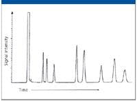
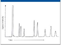
Figure 1: Hypothetical isothermal gas chromatogram.
Understanding Basics of Gas Chromatography Separations
Certainly a number of superb chromatographers still exist, but there are other less capable practitioners,too many of whom are blissfully unaware of their deficiencies. Many of these are highly respected scientists using GC as a tool without realizing that their lack of basic knowledge affects the qualitative and quantitative validity of their results. Ideally, in the classroom environment, we can create situations where they themselves discover their deficiencies, after which most of them promptly take corrective actions. Toward this goal, it can be useful to project an isothermal chromatogram (Figure 1), and pose the question "why is each peak wider than its predecessor?" Many attribute this phenomenon to diffusion: "The longer the solute is in the column, the longer it is subjected to diffusion, ergo the longer the chromatographing band, and the wider the peak." The fallacy of this assumption can be quickly established by pointing out that every solute spends the same time in gas phase (where diffusivity ranges from approximately 0.15 to 0.7 cm2/s), and the slower moving solutes spend longer times in stationary phase (where diffusivity is usually less than 10-6 cm2/s). This means that every solute has suffered essentially the same degree of longitudinal diffusion, all in the gas phase, and there must be some other reason that each successive peak is broader. At this point, it is normal to see many attendees begin to exhibit a heightened interest. This is the time to introduce the concept that it is the Kcs, the solute distribution constants at the time of detection that exercise the major effect on peak conformation. Solutes are conducted from the end of the column to the detection zone only by the carrier gas flow as depicted in Figure 2.

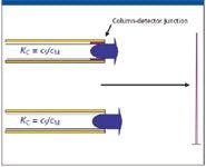
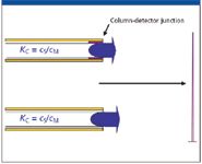
Figure 2: Concept of the solute distribution constant, Kc;cs = concentration of the solute in the stationary phase; cm = concentration of the solute in the mobile (gas) phase.
The solute Kc defines the ratio of the solute concentrations in the stationary phase, cS (where there is no forward motion) compared with that in the mobile phase, cM (where it is continuously swept forward toward the detector), that is, Kc = cS/cM. If the Kc is small at the time the solute approaches the column–detector junction, most of the solute is in mobile phase and is rapidly conducted to detection, producing a peak of short duration and high intensity (Figure 3). If the Kc is large as it approaches this junction, only a small amount is in mobile phase; most is in stationary phase, immune to the forward impetus of carrier flow. As those molecules in mobile phase are swept to detection, more molecules are released from the stationary phase to maintain the equilibrium Kc. Solutes with large Kcs at the time of detection are more slowly dribbled from the column end to the detector, resulting in long-duration low-intensity peaks. Programmed temperature runs are constantly changing solute Kcs, and there is no easy way to tell to what degree of the sharpness of a given peak is a function of the column efficiency, versus the Kc at the time of detection.

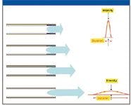
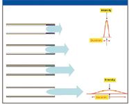
Figure 3: Resultant band broadening as solute is eluted from a column.
Our inability to differentiate these two roles mean that the measurement of column efficiency, retention factors, separation factors, and the like made in programmed mode are of scant value; most such measurements must be made in isothermal mode. Separation efficiency in terms of resolution, such as Trenzahl, can of course be measured in programmed runs.
While it is often possible to separate merged peaks in the detector, our purpose here is to accomplish separation in the column, which is enhanced by sharp narrow peaks.
Figure 4 illustrates the importance of peak sharpness on the separation of two solutes. Retention factors (k) and separation factors (a) are considered constant, and only the sharpness of the peaks — which is mainly affected by the column, the injection efficiency, and operational parameters — varies. It is possible to get more separation than is required — overkill — introducing the possibilities for shorter analysis times. In most laboratories, saving time means saving money.


Figure 4: Illustration of the degree of peak sharpness. Retention factors (k) and separation factors (α) are considered constant.
Injection technique or injection efficiency plays a large role in the length of the band beginning its passage through the column. As bands proceed through the column, they are lengthened by longitudinal diffusion, which as we have seen, occurs almost exclusively in the mobile phase. Each solute spends the same time in mobile phase to reach any given point in the column. Hence, the length of a band during the chromatographic process is a function of its position in the column (see Figure 5). If the efficiency of the injection process can be improved, bands will be shorter, and the shorter the band at the column exit, the sharper the peak, all other factors being constant.

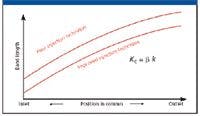
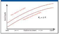
Figure 5: Influence of injection technique on band length. β is the phase ratio.
Still confining our thoughts to isothermal analyses, let us now consider the effect of the analytical temperature on component separations. Separation in GC is achieved during interphase mass transport; that is, only in the cS-to-cM mass transport step. This is usually referred to as mass transfer. Moving something from a gas phase into a liquid phase involves penetration of the surface layer, which is under tension, and dispersion into the liquid phase. In surface chemistry, mass transfer implies that both of these steps have been taken into account. To the best of the author's knowledge, GC theory does not consider the extra energy required to penetrate the surface film. Accordingly, I use the term "mass transport." In this one step, solutes are differentiated on the basis of their "net vapor pressures," that is, their intrinsic vapor pressures, increased by the column temperature, and decreased by the sum of all interactions between that solute and that stationary phase under this particular set of conditions.
Consider the equilibrium distribution of a solute, boiling point approximately 150 °C, at very low temperature (Figure 6, upper left). At low temperature, Kc is immense, and essentially all of the solute is in the stationary phase and only a few molecules are in the mobile (gas) phase. If the temperature is greatly increased (Figure 6, upper right), essentially all of the solute is in the mobile phase and only a trace is in the stationary phase. In both cases, interphase mass transport will occur, but the molecular distribution of the solute is so heavily skewed toward one phase that the number of transitions, cS-to-cM and cM-to-cS, per unit time, is seriously limited — the frequency is low. Somewhere between these two temperature extremes, there is a temperature where the equilibrated distribution of solute molecules between the two phases encourages a maximum transition frequency (lower middle of Figure 6). An isothermal separation at that temperature would yield the best possible separation of this solute from its near neighbors. It would show some discrimination against solutes whose net vapor pressures were slightly higher or slightly lower, and greater discrimination against solutes whose net vapor pressures were still higher or still lower. But for this solute, the temperature is ideal. A major advantage of temperature programming is that each solute spends some time at and near its ideal temperature; the slower the rate of programming, the longer time each solute spends under those conditions, and the better the separation — but the longer the analysis time.


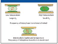
Figure 6: Schematic of interphase transitions at low, high, and optimum temperature. The intensity of the green color depicts the relative concentration of solute in the two phases.
We are now ready to consider the progression of an injected solute through the column. Immediately after injection, each solute partitions between the two phases in accordance with its distribution constant, Kc (Figure 7, top). The equilibrium distribution is continuously disturbed by the forward movement of the carrier gas, which depletes the gas-phase concentration at the rear of the chromatographing band while it advances over virgin stationary phase at the front of the band (Figure 7, center). Immediately after injection, the solute bands are all intermixed, but each solute band is constantly disappearing at the rear and being reestablished at the front (Figure 7, bottom). The more volatile (low Kc) solutes volatilize more rapidly and soon dominate the front of the moving band, while the less volatile (high Kc) solutes dominate the rear. As this process continues, the mixture of slowly separating solute bands eventually separates into individual bands.

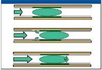

Figure 7: Schematic of the progression of an injected solute through a column.
By this time, those readers who recognize that their GC skills can benefit from an understanding of basic GC principles are ready to proceed to considerations of the van Deemter treatment, and on into more advanced topics including the rationale for changes in peak elution sequences that often accompany the installation of a "replacement" column. Those topics, however, lie beyond the scope of this paper.
Acknowledgments
The author would like to thank Konrad Grob for an initial reading of this manuscript, and for valuable suggestions. He also would like to thank Rudolf Kaiser, Leon Blumberg, Matthew Klee, Patrick Sandra, Frank David, and Ron Majors for suggestions and support.
"Column Watch" Editor Ronald E. Majors is business development manager, Consumables and Accessories Business Unit, Agilent Technologies, Wilmington, Delaware, and is a member of LCGC's editorial advisory board. Direct correspondence about this column to "Sample Prep Perspectives," LCGC, Woodbridge Corporate Plaza, 485 Route 1 South, Building F, First Floor, Iselin, NJ 08830, e-mail lcgcedit@lcgcmag.com
References
(1) G. Guiochon and C.L. Guillemin, Quantitative Gas Chromatography for Laboratory Analyses and On-Line Process Control (Elsevier, Amsterdam, 1988), p. 249.
Dr. Walt Jennings is Professor Emeritus of the University of California, Davis. He is co-founder of J&W Scientific, now part of Agilent Technologies, Folsom, CA and also a co-founder of Air Toxics, Inc., Folsom, CA. His e-mail address is: waltj@pacbell.net


TD-GC–MS and IDMS Sample Prep for CRM to Quantify Decabromodiphenyl Ether in Polystyrene Matrix
April 26th 2024At issue in this study was the certified value of decabromodiphenyl ether (BDE 209) in a polystyrene matrix CRM relative to its regulated value in the EU Restriction of Hazardous Substances Directive.

 and Dr. Valérie Agasse (right) of the University of Rouen. Photo Credit © Pascal Cardinael and Valérie Agasse.")
Inside the Laboratory: The Chromatography Laboratory at the University of Rouen
April 18th 2024In this edition of “Inside the Laboratory,” Pascal Cardinael and Valérie Agasse of the University of Rouen in Mont‑Saint-Aignan, France, discuss their laboratory’s work with miniaturizing gas chromatography (GC) columns and systems to improve on-site air analysis of volatile organic compounds (VOCs).