Statistics for Analysts Who Hate Statistics, Part IV: Clustering

Part IV of this article series takes a closer look at clustering. Clustering is a useful way of grouping your samples to identify those that are most similar, and is perhaps easier to interpret than principal component analysis, because it provides a single figure retaining most of the initial information.

Clustering can be very useful for observing your data when the sample dimensionality is large, which is a barbarian term meaning that diversity among your samples may be wide. In that case, the space reduction provided by principal component analysis (PCA) is not always convincing, because the simplification provided by a single two-dimensional plot is erasing too much information. Clustering allows you to preserve more information.

Clustering is a way to classify observations (1). Like PCA, it is an unsupervised method, meaning that no previous knowledge of the data set is required. Clustering methods classify observations defined by variables. For instance, hierarchical cluster analysis (HCA) will first join together the observations that are most similar, then the ones that are a little less similar, then the ones less similar, and so on, until the most dissimilar observations are clustered.

There are several ways to evaluate the similarity between the observations: It will be evaluated by the “measurement” of a distance. The simplest one is the Euclidean distance: For a two-dimensional problem (observations defined by two variables), the Euclidean distance is the one you would measure with a ruler, on a paper where you would have plotted your observations. As you probably learned when you were younger, Euclidean distance is the square root of the sum of squares of distances measured on each axis. There are also several ways to cluster the observations. One that is easily understandable is Ward’s aggregation method: The distances between all observations are measured and the closest two are clustered; they are replaced by an average point (the barycenter) that is now compared to all other points, and so on.

I will explain this approach with a simple case where only two variables are sufficient to describe the problem. In Figure 1, I have represented my “friends network.” For the purpose of simplicity, I have retained only those close to France (France, England, and Switzerland). As you can see in the figure, I have friends close by, as well as in other places where I have lived or where my friends have moved. You can describe this map very simply using a data table in which the “observations” will be me and my friends, and the variables will be latitude and longitude as given by a GPS locator. Because one degree of latitude and one degree of longitude represent different distances, it is preferable to normalize the data (center and reduce latitude and longitude). Now if we analyze this data table with HCA, we will obtain Figure 2, which displays the hierarchical links. This plot is called a dendrogram. The abscissa basically reflects geographical distance between all the people in my network. You can see very short links between the people living close to each other, and longer links for those living at a distance. Three main groups appear, with me and (geographically) closer friends in one group, all those in the east of France in another group, and T in England, alone in his group.

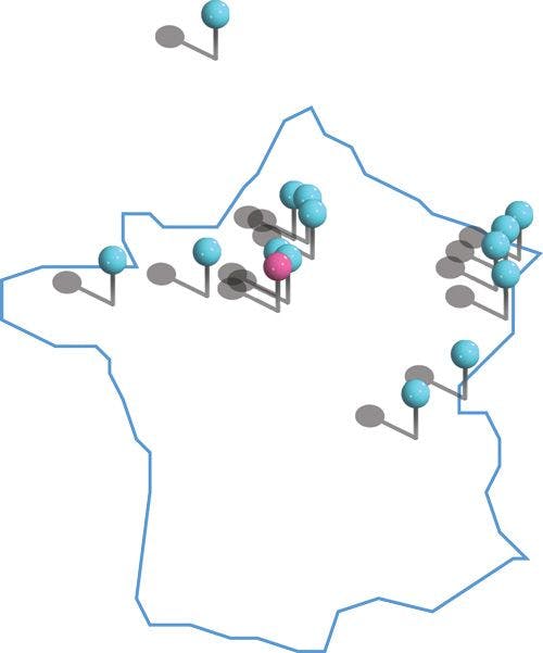
Figure 1: My French network of friends (blue pins; I am in pink).

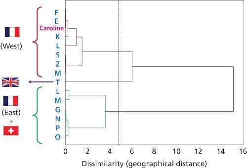
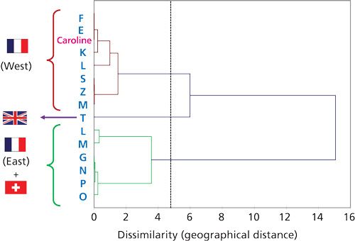
Figure 2: Dendrogram of my French network of friends based on latitude and longitude.

Depending on the software used and settings selected, a “cutting line” may appear on the figure, to define clusters of observations with a “define similarity” level. You may choose to trust the software in deciding where the cutting line should be placed; this approach  will ensure that the definition of groups among your samples will be completely objective. For my part, I’d rather trust my knowledge of samples and understanding of the chemistry to decide where the cutting line should be placed, thereby introducing some subjectivity in the decision. In the friends network example, I could have decided to displace the cutting line to shorter geographical distance, so as to separate the people in Alsace from those around Lyon (Eastern region) or to separate the people in Brittany from Paris and Orleans locations.

The definition of clusters based on the cutting line of the dendrogram is also useful when deciding how to group clusters in PCA plots. PCA plots of observations often show ellipses circling groups of observations that are supposedly similar. One objective way of drawing the ellipses is to establish the groups based on cluster analysis (2,3).

Let us now apply HCA to a chromatography problem. If we have analyzed a number of samples (observations) with the same chromatography method, we may use the chromatographic data (for instance, peak areas of identified species or the full detector trace) as variables. HCA will provide a simple summary of chromatographic differences.

As an example, I will tell you about a study I participated in some years ago. In my laboratory, there is a wide interest in samples extracted from natural products. The extracts are usually analyzed with a variety of chromatographic methods to retrieve “fingerprints” of the samples. Clustering is a simple way to compare these chromatographic fingerprints to detect similar or dissimilar samples. In this example (4), we were interested in resins retrieved from coniferous plants from different botanical and geographical origin. Looking at the liquid chromatography–mass spectrometry (LC–MS) chromatograms and comparing them visually is an appropriate approach when the samples are not too numerous, and when the chromatograms are simple, but not when the sample number increases or when chromatograms are complex. In Figure 3, it is easy to see that some resins from different botanical origin produced similar LC–MS chromatograms (Boswellia and Canarium resins), while other botanical origins may produce different resins (among the Commiphora resins).

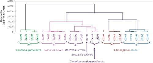
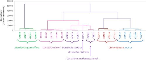
Figure 3: Hierarchical cluster analysis to compare several resin extracts from different botanical and geographical origins based on liquid chromatography–mass spectrometry (LC–MS) chromatograms.

To conclude, I should also point out that clustering calculations is a very rapid process, much more so than calculating a PCA. Visually, the dendrogram is simple and is understandable by nonspecialists (short lines link “close” or “similar” observations, while long lines link “dissimilar” observations), which makes it a good tool for communication.

In the next article of this series, we will start looking at supervised data analysis methods with discriminant analysis.

References

1. D.L. Massart, J. Smeyers-Verbeke, and Y. Vander Heyden, LCGC Europe19, 99–103 (2006).
2. C. West and E. Lesellier, J. Chemometrics26, 52–65 (2012).
3. K. Le Mapihan et al., J. Chromatogr. A1030, 135–147 (2004).
4. B. Rhourrhi-Frih et al., J. Chromatogr. A1256, 177–190 (2012).

Caroline West is an assistant professor at the University of Orléans, in Orléans, France. Direct correspondence to: caroline.west@univ-orleans.fr.