From Detector to Decision, Part IV: Demystifying Peak Integration

Most quantitative analysis in chromatography is performed based on the peak area, the integrated area underneath the curve defining a peak. There are many variables and settings in a data system that can impact this determination. In this installment, we will examine several of the common parameters that can affect automated peak integration and the resulting peak areas. We will consider how the data system detects the beginning and end of the peak, how it determines the peak maximum, how real peaks are differentiated from noise, and how signals at individual time intervals are summed to generate the peak area. We will also briefly look at techniques for determining the areas of unusually shaped peaks.

In previous installments, we have discussed what happens between the generation of signal by the detector and the appearance of a chromatogram on the screen or in a report. We discussed the basics of how the detector signal is converted into data and reports by the data system, how modern data systems automate operation of the instrument, and calibration techniques (1–3). We now take a step back from calibration and look at peak integration, which is one of the most important functions that happens behind the scenes.

Calibration and quantitative analysis based on peak areas are not possible without integration, and we will see that, while integration is now performed automatically by the data system, there are several parameters that should be understood by the user to ensure reliable and reproducible results.

What is Integration?

On a two-dimensional plot, such as a line or a traditional chromatogram, integration involves calculating the sum of the y-axis data points over a chosen range of the curve. A typical equation describing an integral is shown in equation 1:

The integral sign and the variables a and b represent that this is a definite integral with lower limit a, and the upper limit b, and the summation occurring between a and b on the x-axis. The function being integrated, called the integrand is f(x). The term dx represents the variable being integrated and can be thought of one slice or data point of that variable. We can also think of the integral as the sum of the y-axis data points, expressed in equation 2 as a summation.

For a chromatographic peak, the limits of the summation or integration are given by the beginning and end of the peak, and the integer increments for the summation are given by each individual data point recorded by the detector.

Why Integrate? Origins of Chromatographic Peaks

Most modern quantitative chromatographic methods use the area underneath a peak, known as the peak area, to ultimately calculate the mass or concentration of each analyte of interest. Calibration techniques, including area percent normalization, response factors, internal standard, external standard, and standard additions were reviewed in a recent column (3). All these techniques rely on the peak area to provide the y-axis data used in plotting the calibration curve or calculating the estimated analyte mass or concentration.

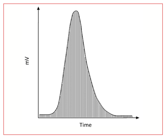
Figure 1 shows a chromatographic peak, divided into slices, to show a simplified graphical example of peak area determination. The peak area is simply the sum, or integral of the signals. The signal is generated, usually as a voltage, by the detector, which is then converted to a series of data points versus time through sampling by an analog to digital conversion, and then transmitted as a digital signal to the data system, where the series of data points is stored in a file for analysis and reporting, including integration.

FIGURE 1: Integration of a peak. Each slice is a data point. Adapted from CHROMacademy, LCGC International’s online learning platform (5).

Main Factors Affecting Integration

There are several detector and data system settings that can impact integration, peak detection and peak areas. A full description of each of these could more than fill a “GC Connections” column, so we will summarize some key points with each and briefly discuss the origins of each of their effects on integration.

The detector data acquisition rate will usually not change the peak area, but it does change the width of each of the slices seen in Figure 1. Threshold is a measure of the change in the slope of the curve seen in Figure 1 (the second derivative of the curve), and is used to determine when the peak starts and stops. A peak width setting can prevent integration of peaks, such as short-term noise spikes, that are too sharp to be analyte peaks. The last two factors, peak shape and peak overlap, are not detector or integrator settings, but they can have a major impact on integration. There still is no universally effective means for precisely and accurately integrating overlapped peaks and separating the overlapped signals.

The units of an integrated peak, as seen in Figure 1 where the y-axis is in mV and the x-axis is sec are: mV × sec. Each slice is a rectangle with the long side (y-axis) in mV and the short side (x-axis) in sec.

Data Acquisition Rate

The data acquisition rate determines the number of x-axis data points for any given period of time on a chromatogram. For a flame ionization detector (FID), a typical data acquisition rate is 20–50 data points/s. If a peak is two seconds wide, then there are 40 data points at 20 points/s. In performing the integration, the signals measured for these 40 data points are summed by the data system, with each signal being multiplied by 1/20 s to give the area of the slice in mV s. If the acquisition rate is 50 data points/s, then there are 100 data points, but each is multiplied by 1/50 s to give the area of each slice. The two peak areas then add the same.

Integration and peak area can be affected by acquisition rate in two situations. First, higher acquisition rate usually leads to increased noise, which may not affect the average peak area determined for multiple samples, but can impact the precision of that average. Second, if the peak is narrow or the acquisition rate is too slow, there may not be enough data points to precisely define the peak. This is most often seen in full-scan gas chromatography–mass spectrometry (GC–MS), where the acquisition rate may only allow a few scans to determine a peak.

Threshold

Examining the peak in Figure 1, in order to determine the beginning and end of the peak and the maximum, for reporting the retention time, the integrator must examine the slope of the curve and determine changes. Before the peak is eluted (to its left on the plot in Figure 1), all we see is baseline, the slope of the curve (first derivative) is zero, and the slope is not changing (second derivative is zero). As the peak starts to rise, the slope becomes positive and is increasing; both the first and second derivatives are positive.

Threshold is a measure of these two derivatives that tells the integrator when the peak starts, and therefore when to start summing the peak area. This is an adjustable parameter that can clearly affect the summed peak area. If the threshold is too sensitive, then noise and baseline may be included in peak areas, and small, spurious peaks due to noise and baseline drift may be integrated. If the threshold is not sensitive enough, then small peaks of interest may not be counted, and peak areas may be slightly low.

As we follow the peak rise, there is an inflection point where the slope is still positive but the change in slope goes to zero and then the slope, while still positive, is decreasing. When the slope and the change in the slope then reach zero, this is the peak maximum and the retention time is recorded. Following the peak maximum, the slope starts to increase in the negative direction, again passing through an inflection point, and eventually both the slope and the change in slope return to zero. This marks the end of the peak, and integration is stopped. Threshold impacts the location where the peak starts and stops, the number of data points used to calculate the peak area, and the peak area itself.

Peak Width

Generally, in chromatography, the peak width increases predictably as retention time increases. In isothermal separations, the peaks get wider and shorter; in temperature programming they are all about the same width, and may get slightly wider with longer retention times (4). The peak width setting on an integrator allows for peaks of unusually wide or narrow peak width to not be integrated, as these are often spurious results and not analyte peaks, or if improperly set can result in too many peaks (such as noise being integrated), or too few (such as some analyte peaks of interest not being integrated). Most data systems today will default this to an appropriate setting based on chromatographic conditions; it may need adjustment if peaks of interest are not integrated, or if too many peaks, including apparent noise spikes, are integrated.

Peak Shape

As seen in Figure 1, most chromatographic peaks are symmetrical, in statistics, representing a Gaussian distribution of mass around the center of mass, which is also seen at the peak maximum. The peak maximum is also the reported retention time. For a symmetrical peak, the retention time also corresponds to the center of mass of the peak and the peak width, discussed above, represents a function of the width at baseline or at half-height, corresponding to the width at the inflection points described above.

Commonly, chromatographic peaks are not symmetrical; they either front, with more of the mass eluting before the peak maximum, or they tail, with more of the mass eluting after the peak maximum. Examples of symmetrical, fronting, and tailing peaks are shown in Figure 2.

FIGURE 2: Symmetrical, fronting and tailing peaks.

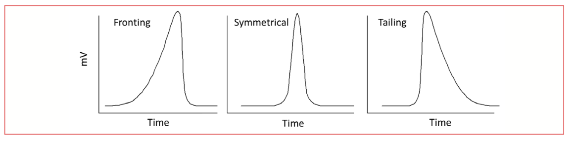
Looking at the fronting and tailing peaks in Figure 2, we immediately see that the front of the fronting peak and the back of the tailing peak have unusual shapes, representing greater mass toward the beginning of the fronting peak and greater mass toward the end of he tailing peak. While, for the same analyte mass, the total peak area is nominally the same as a symmetrical peak, these peaks present several problems for the integrator.

As discussed above, the starting and ending points of the peak for integration are determined by changes in the slope of the curve. As seen in Figure 2, the curve at the start of the fronting peak has a different shape than the symmetrical peak; if the integrator is optimized for detecting the expected slope change for the symmetrical peak, it may not accurately detect the start of the fronting peak. Likewise, this situation would arise for detecting the end of the tailing peak. This can reduce both precision and accuracy of integration.

Peak shape also impacts the accuracy of retention time determination. Note in Figure 2 that the maximum of the fronting peak is shifted to a later retention time for the fronting peak, and to an earlier time for the tailing peak. By inspection, we also see that since the peak is not symmetrical on either side of the peak maximum, that the maximum no longer represents the center of mass. Further, this shift in the peak maximum becomes more pronounced as the tailing or fronting increases. In the rare case where the amount of tailing or fronting is reproducible, the retention time shift may not be a problem, as the retention time, although not representative of the center of mass of the peak, will still be reproducible. In gas chromatography, the situation, especially with tailing, where the amount of tailing varies, usually increasing with time and more column or inlet use, the retention time will vary, becoming shorter as the amount of tailing increases.

Conclusions

Peak integration is one of the many operations that occurs in the background on today’s modern gas chromatographs and in their data systems. The peak area values shown in an area percent report are a function of the mass or concentration of analyte that has passed through the detector over a given time, as determined by an integration function in the data system. This integrator and the user must perform several functions to determine the peak area: detecting the start and end of the peak, the limits of integration; determining whether the peak is an analyte peak, baseline drift or noise; and accounting for variations in integration and retention time determination for asymmetrical peaks. These operations, while in the background, are often not simple, and failing to pay attention to them may cause loss of both accuracy and reproducibility in quantitative analysis.

References

(1) Snow, N. H. From Detector to Decision: How Does the GC Instrument Generate Your Data? LCGC North Am. 2020, 38 (9), 496–500.

(2) Snow, N. H. How Can We Run a Gas Chromatograph from Anywhere? LCGC North Am. 2020, 38 (11), 601–605.

(3) Snow, N. H. From Detector to Decision, Part III: Fundamentals of Calibration in Gas Chromatography. LCGC International 2024, 1 (1), 12–16.

(4) Snow, N. H. Temperature Programmed GC: Why Are All Those Peaks So Sharp? LCGC North Am. 2019, 37 (7), 450–456.

(5) Watson, D. The What, When, and How of Peak Integration: Part 1. What. CHROMacademy. https://www.chromacademy.com/channels/data-analysis/principles/the-what-when-and-how-of-peak-integration-part-i-what/ (accessed February, 2024).

About the Author

Nicholas H. Snow is the Founding Endowed Professor in the Department of Chemistry and Biochemistry at Seton Hall University, and an Adjunct Professor of Medical Science. During his 30 years as a chromatographer, he has published more than 70 refereed articles and book chapters and has given more than 200 presentations and short courses. He is interested in the fundamentals and applications of separation science, especially gas chromatography, sampling, and sample preparation for chemical analysis. His research group is very active, with ongoing projects using GC, GC–MS, two-dimensional GC, and extraction methods including headspace, liquid–liquid extraction, and solid-phase microextraction.