The Gradient Delay Volume, Part III: Practice – Effects on Throughput

The concept of gradient delay volume (GDV) in liquid chromatography (LC) poses challenges for both beginners and experienced practitioners. The GDV, which affects the arrival time of mobile phase composition changes at the column inlet, can have a significant impact on method throughput, influencing the time required for mobile phase changes at both the beginning and end of the LC method. Different pump designs and column characteristics affect efficient use of the available analysis time, as well as overall throughput. Notably, achieving repeatable equilibration, rather than full equilibration of LC columns following mobile phase gradients, is often sufficient for many LC applications, which can also be leveraged to increase method throughput.

In my interactions with people learning about various aspects of liquid chromatography (LC), I find that the concept of gradient delay volume (GDV) is one of the most difficult ideas to grasp and apply in practice. I find this to be the case both for true beginners—students who are just learning the basics of LC—and for more experienced scientists who have always dealt with GDV, knowingly or unknowingly, but are perhaps having to think about its impacts on their work in new ways. The GDV concept has been important since the very first time LC separations involving changes in mobile phase composition were made during an analysis. This is a phenomenon now know as a gradient elution separation. However, given the various ways that GDV can impact the practice of LC, and that we continue to see changes in commercial instrumentation that affect the way we interact and think about GDV, I think a dive into the details is warranted here.

In the last two installments of “LC Troubleshooting,” I reviewed the basic elements of the GDV concept and discussed how we understand that GDV affects characteristics of LC separations from a theoretical point of view. I then discussed the practical implications of these ideas, with an emphasis on how the differences in GDVs between instruments can impact how a particular method will function on those instruments. In this month’s installment, I will discuss the impact of GDV on method throughput, since GDV leads to a time where we need to wait for changes in the solvent composition delivered to the LC column at both the beginning and the end of a gradient elution method.

The gradient delay volume is commonly referred to by others as the gradient dwell volume, or sometimes just dwell volume. I prefer the inclusion of “gradient” to make it clear what we are talking about, and I prefer “delay” over “dwell,” because “delay” communicates one of the most important impacts of GDV—that it delays the arrival of a programmed change in mobile phase composition at the column inlet. Nevertheless, from my point of view, “gradient delay volume” and “gradient dwell volume” refer to the same thing.

Finally, readers interested in learning more about GDV will not have a hard time finding good resources, and are encouraged to consult them. A short list includes several articles in LCGC Magazine and the book by Snyder and Dolan that is focused entirely on gradient elution LC (1). The relatively recent books, edited by Stavros Kromidas, have rich sections written by major instrument vendors that explain in some detail the software- and hardware-oriented approaches they have taken to effectively achieve variable GDV in their instruments (2,3). Searching the “LC Troubleshooting Bible” website (https://lctsbible.com/) for the keyword “dwell volume” will immediately return about a dozen articles from the last 20 years.

Changes in Mobile Phase Composition at the Beginning and End of a Gradient Elution Method

In the previous two installments in this series, the focus of the impact of GDV has been on its effect on the arrival of the change in mobile phase composition at the column during the early stages of the gradient. However, we should not overlook the impact of the GDV on what happens at the end of the gradient. Here, when the pump is instructed to change the mobile phase composition back to the initial level used in the gradient (ϕ_i), we have to wait for the “strong solvent” used in the gradient to be washed out of the pump and other components leading to the column. Only when the mobile phase composition used as the initial level in the gradient actually reaches the column can the column actually start equilibrating with this mobile phase in preparation for the next analysis. The relationship between the solvent gradient program—that is, the instructions we give to the pump—and what the column actually experiences at the inlet is illustrated in Figure 1.

FIGURE 1: Solvent program instruction delivered to the LC pump (solid line), and the mobile phase composition observed at the column inlet (dashed line). Adapted from reference (4).

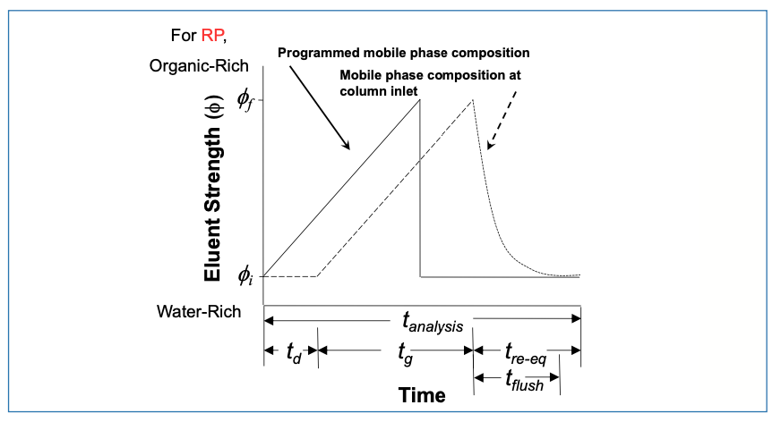
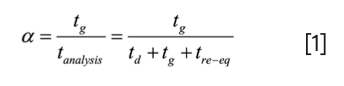
The delay in the arrival of a change in composition on the front side of the gradient is t_d = V_d/F. On the back side of the gradient, the time required to flush the strong solvent from the pump and connecting components is t_flush. Given the exponential profile of this flushout, for practical purposes, we assume that t_flush is about 2 × t_d, or t_flush = 2 ^. V_d/F. Additionally, we see that t_re-eq is a bit longer than t_flush. Here, we define the re-equilibration time t_re-eq as the time required to re-equilibrate the column, including t_flush. So, we understand that the difference between t_re-eq and t_flush is the time we allow the column to equilibrate with the mobile phase composition used as the starting point in the gradient (ϕ_i). Later on in this installment, I’ll discuss more of what constitutes “enough” time for re-equilibration of the column itself; for the remainder of this section, we’ll assume that two column volumes of equilibration is enough, such that t_re-eq = t_flush + 2 ^. V_m/F, where V_m is the dead volume of the column. Finally, when thinking about the throughput of analyses involving gradient elution, it is useful to define a fraction α that quantifies the portion of the analysis time that is actually used for separating things under solvent gradient conditions (5) (nominally, t_g; peaks can elute during t_d as well, but we assume here that elution during the isocratic pre-gradient phase is generally not as useful as elution during the actual gradient).

Having defined α and all the times involved, we can think about the effects of different variables on throughput and the fraction of the analysis time that is actually used for separation, including V_d, F, and V_m. Table I shows some different combinations of these variables, along with a description of where these combinations are found most often in practice. First, in Scenario A, we see that when using a modern binary pump characterized by a small GDV, a relatively short, narrow column, and a reasonably fast gradient time of 2 min, the fraction of analysis time that is the gradient time is about 70%, which is not too bad. Now, if we use the exact same conditions in Scenario B, but change the pump to a quaternary, low-pressure mixing design characterized by a large GDV, we see that α drops to around 40%. If there is no other choice due to resource constraints, then this is how it has to be, but using less than 50% of the analysis time for the gradient separation is far from optimal. In Scenario C, we suppose that the focus is more on performance as measured by peak capacity or resolution, as derived from the use of a longer column. If we stick with the same pump as in Scenario B, the α value increases only marginally, mainly because when we move to the longer column, we have to use a lower flow rate to avoid going over the pressure limit of the system, which, in turn, leads to larger values of t_d and t_re-eq. The takeaway from Scenario D is that efficient usage of the analysis time (as measured by a large α) is indeed possible, even with an older pump with a large GDV; however, this requires much higher flow rates, and thus, a larger diameter column. The high flow rate reduces t_d and t_re-eq, while maintaining a gradient slope, similar to that in Scenario A. Scenario E illustrates what happens when we try to use a modern, short, narrow column with an old quaternary pump with a large GDV. The α value drops to around 24%, which will be unacceptably low in most cases.

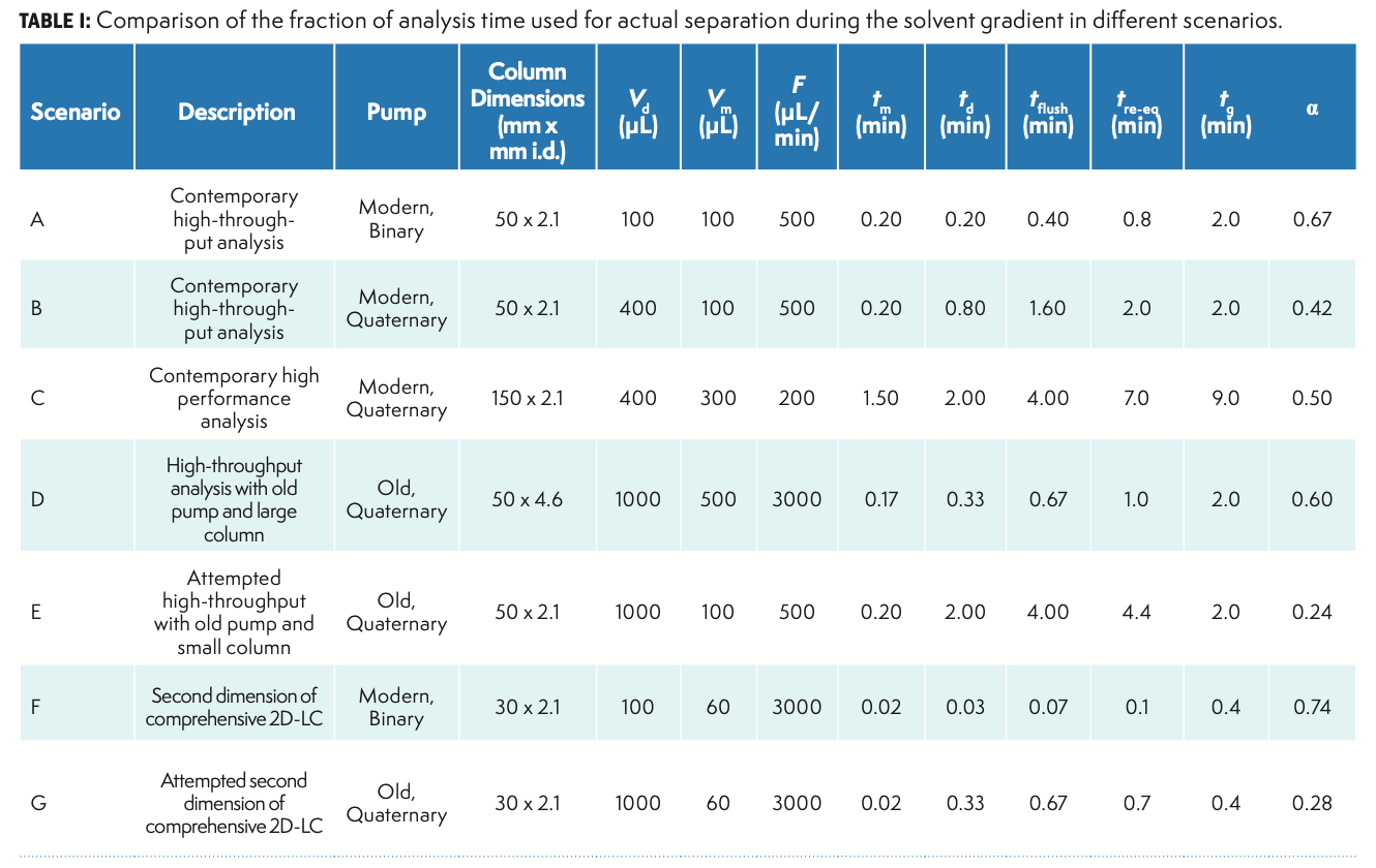
The final two scenarios in Table I (F and G) are relevant to gradient elution conditions used in the second dimension of comprehensive 2D-LC separations. In this case, the performance requirements are relatively unusual—very short analysis times on the order of 30 s are highly valuable. Scenario F shows that if a short, narrow column is used, along with a modern binary pump and a relatively high flow rate, the α fraction can actually be quite high at around 70%, which is similar to what we see with conventional 1D-LC separations. However, if we imagine trying to do the same 30-s separations using an old quaternary pump, the α value drops again to an unacceptably low 28%. This application effectively requires the use of modern binary pumps.

How Long Do We Actually Need to Re-Equilibrate the Column?

In the mid-2000s, I began looking into this question deeply, along with Adam Schellinger and Peter Carr, motivated by our interest in superfast gradient elution conditions along the lines of Scenario F in Table I (6–8). One of the most important things we learned from our work at that time is that, when talking about re-equilibration of LC columns following a mobile phase composition gradient, we really have to make a distinction between two different types of equilibration:

1. A state of repeatable equilibration. In this case, the column is not actually fully equilibrated with the initial mobile phase used in the gradient before starting the next analysis, but the condition of the column is consistently achieved between analyses, such that highly repeatable retention times are observed.
2. A state of full equilibration. In this case, the column is fully equilibrated, as indicated by the observation that retention time observed in the gradient elution method is independent of the re-equilibration time between analyses.

Our realization at the time was that for many applications of gradient elution methods in LC, we care far more about having highly repeatable (that is, precise) retention times than we care about starting with a column that is in a fully equilibrated state.

Once we realized the importance of this distinction between states, we found that for reversed-phase separations of small molecules, it usually does not take more than two column volumes (or two dead times of flushing with ϕi) to get to a state of repeatable equilibration. For large columns operated at conventional flow rates (for example, a 150 mm x 4.6 mm i.d. column operated at 2 mL/min), this is about 1.5 min. But for short columns at high flow rates, this can be remarkably short at just a few seconds (for example, as in Scenario F in Table I).

This finding has since been confirmed by other groups for reversed-phase separations (9,10), and also for other modes of separation, such as hydrophilic interaction liquid chromatography (HILIC) (4,11). Frankly, modern comprehensive 2D-LC separations would not exist as we know them today if it were not possible to repeatedly equilibrate LC columns in a matter of seconds (12).

Summary

In this installment of “LC Troubleshooting,” I have discussed the effects of gradient delay volume (GDV) on the throughput of LC methods that involve mobile phase composition gradients. While we very often focus on the impact of the gradient delay time and its effects on selectivity and resolution, as discussed in last month’s installment, the more important impact of GDV on throughput occurs at the end of the method, where we instruct the LC to return the mobile phase to the initial condition used in the gradient. Understanding the interactions between pump characteristics, column characteristics, and other method parameters and performance goals is useful when developing a new method with throughput in mind, troubleshooting variations in retention time, and optimizing existing methods to improve throughput.

Case Study Corner

This month, I am rolling out a new feature in the “LC Troubleshooting” column, The “Case Study Corner.” Here, I will provide a short description of a real problem I’ve observed, and ask readers to send me their diagnosis of the root cause of the problem and a proposed solution. The first person to propose the correct diagnosis and solution will receive an “Analytically Speaking” podcast coffee mug. In a subsequent installment, I will then discuss the correct diagnosis and solution in some detail. I encourage educators and lab managers to consider assigning these case studies as “homework” to their students and scientists to help them develop their troubleshooting skills. Enjoy!

Case Study #1

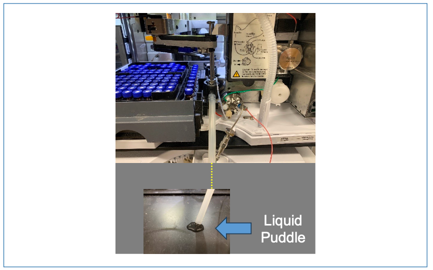
The focus of this month’s case study is a problem with a LC autosampler, and this time, we have two major troubleshooting clues. The first clue is the pressure trace measured at the LC pump, as shown in Figure A. Here, I’ve included data from two full analysis cycles in the plot, and we see that the pressure drops dramatically at the end of the first analysis, but then rises quickly to the nominal operating pressure very early in the second analysis. When I was observing this instrument, I saw that this pattern was repeated over tens of injections. The second clue is that I observed a puddle of liquid on the benchtop in front of the LC, as shown in Figure B. This particular sampler involves a flow through needle design (Agilent G4226A). Readers are welcome to email me at dstoll@gustavus.edu with clarifying questions, in addition to sending their proposed diagnoses and solutions to the problem.

FIGURE A: Pressure profiles measured at the pump over two analysis periods; sample injections were made at 0, 3, and 6 min.

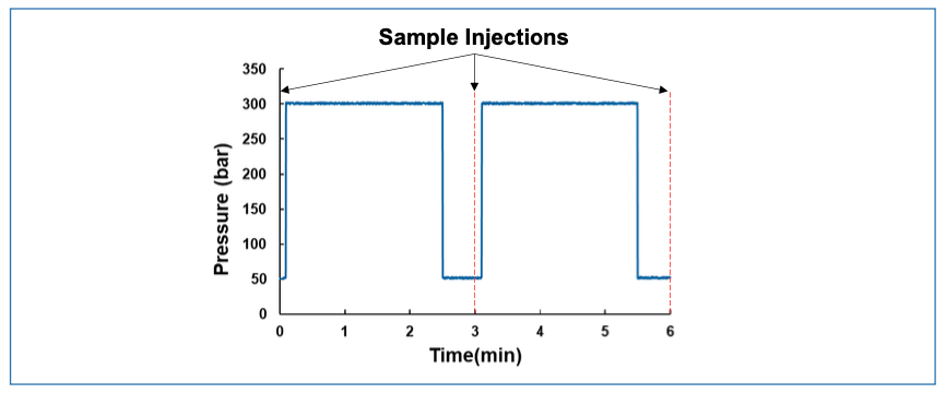
FIGURE B: Picture of the sampler in question and the puddle of liquid observed on the benchtop in front of the instrument.

References

(1) Snyder, L. R.; Dolan, J. W. High-Performance Gradient Elution: The Practical Application of the Linear-Solvent-Strength Model; John Wiley, 2007.

(2) Gradient HPLC for Practitioners: RP, LC-MS, Ion Analytics, Biochromatography, SFC, HILIC; Kromidas, S., Ed.; Wiley-VCH, 2019.

(3) Optimization in HPLC: Concepts and Strategies; Kromidas, S., Ed.; Wiley-VCH, 2021.

(4) Stoll, D., R.; Seidl, C. Column Re-Equilibration Following Gradient Elution: How Long Is Long Enough? Part I: Reversed-Phase and HILIC Separations of Small Molecules. LCGC N. Am. 2019, 37 (11), 790–795.

(5) Horváth, K.; Fairchild, J. N.; Guiochon, G. Generation and Limitations of Peak Capacity in Online Two-Dimensional Liquid Chromatography. Anal. Chem. 2009, 81 (10), 3879–3888. DOI: 10.1021/ac802694c

(6) Schellinger, A.; Stoll, D.; Carr, P. High Speed Gradient Elution Reversed-Phase Liquid Chromatography. J. Chromatogr. A 2005, 1064 (2), 143–156. DOI: 10.1016/j.chroma.2004.12.017

(7) Schellinger, A. P.; Stoll, D. R.; Carr, P. W. High-Speed Gradient Elution Reversed-Phase Liquid Chromatography of Bases in Buffered Eluents - I. Retention Repeatability and Column Re-Equilibration. J. Chromatogr. A 2008, 1192 (1), 41–53. DOI: 10.1016/j.chroma.2008.01.062

(8) Schellinger, A. P.; Stoll, D. R.; Carr, P. W. High Speed Gradient Elution Reversed Phase Liquid Chromatography of Bases in Buffered Eluents - II. Full Equilibrium. J. Chromatogr. A 2008, 1192 (1), 54–61. DOI: 10.1016/j.chroma.2008.02.049

(9) Rogatsky, E.; Cruikshank, G.; Stein, D. T. Reduction in Delay Time of High‐dwell Volume Pumps in LC‐MS Applications Using Short‐term Low‐ratio Split Flow. J. Sep. Sci. 2009, 32 (2), 321–327. DOI: 10.1002/jssc.200800393

(10) Tomasini, D.; Cacciola, F.; Rigano, F.; Sciarrone, D.; Donato, P.; Beccaria, M.; Caramão, E. B.; Dugo, P.; Mondello, L. Complementary Analytical Liquid Chromatography Methods for the Characterization of Aqueous Phase from Pyrolysis of Lignocellulosic Biomasses. Anal. Chem. 2014, 86 (22), 11255–11262. DOI: 10.1021/ac5038957

(11) Heaton, J. C.; Smith, N. W.; McCalley, D. V. Retention Characteristics of Some Antibiotic and Anti-Retroviral Compounds in Hydrophilic Interaction Chromatography Using Isocratic Elution, and Gradient Elution with Repeatable Partial Equilibration. Anal. Chim. Acta 2019, 1045, 141–151. DOI: 10.1016/j.aca.2018.08.051

(12) Stoll, D., R.; Leme, G. M. Chapter 4: Instrumentation for Two-Dimensional Liquid Chromatography. In Multi-Dimensional Liquid Chromatography: Principles, Practice, and applications; CRC Press, 2022.

About the Author

Dwight R. Stoll is the editor of “LC Troubleshooting.” Stoll is a professor and the co-chair of chemistry at Gustavus Adolphus College in St. Peter, Minnesota. His primary research focus is on the development of 2D-LC for both targeted and untargeted analyses. He has authored or coauthored more than 75 peer-reviewed publications and four book chapters in separation science and more than 100 conference presentations. He is also a member of LCGC’s editorial advisory board. Direct correspondence to: LCGCedit@mmhgroup.com