Nonclassical Methods and Opportunities in Comprehensive Two-Dimensional Gas Chromatography

A typical schematic diagram of the GC×GC instrument is shown in Figure 1a. This is the system developed in our laboratory, which pioneered the use of cryogenic methods for modulation. A moving cryotrap affects the modulation process (see the following). The separation advantage of GC×GC is represented simply in Figure 1b. The one-dimensional (1-D) GC experiment suffers considerable overlap of peaks (Figure 1b), and heart-cutting methods are able to relieve this limitation for specific regions of the chromatogram (Figure 1c) by passing them to a second column for subsequent separation. This cannot be applied easily for all neighboring regions; however, the innovative GC×GC approach is able to apply a continuous two-dimensional (2-D) separation to the total sample by rapidly modulating (collecting and reinjecting) the first-dimension (¹D) column effluent into the second-dimension (²D) column (Figure 1d). Thus, the technique produces a 2-D separation with peaks separated over a 2-D plane, which has considerably more "separation space." The classical GC×GC experiment incorporated a conventional length (~30 m) ¹D column interfaced to a short ²D column, typically 1–1.5 m long. The inner diameter ratio of the two columns was about 2–3, and the modulation period (P _M ) was about 4–7 s. This period was selected based upon the peak width generated on the first column, such that the modulation ratio [ratio of peak width at base (w_b) to modulation period] M_R was about 3–4.

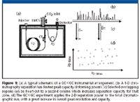
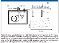
Figure 1

Figure 2 presents the process used to generate first the modulated peaks, then the data manipulation, and finally presentation to a 2-D plot. Here, the relative peak widths on each dimension are represented, and the modulation period leads to about seven modulated peaks, which is probably oversampling of the ¹D peak. Each ²D peak is a separate chromatogram on the second column, and data transformation treats this somewhat like a data matrix determined by each of these chromatograms. This is shown in an offset diagrammatic fashion in Figure 2. There are a few ways to operate the first column to satisfy these conditions, and a short but very thick film column also will achieve the desired first peak width that allows multiple sampling of the peak. As far as the ²D column is concerned, it really is only concerned about the elution temperature (T_e) of the compounds as they pass from the ¹D column to the ²D column. T_e determines the retention factor (k = t'_R/t_M, where t'_R is the adjusted retention time, and t_M is the dead time or holdup time of the compounds on the ²D column, based upon carrier flow rate [L/t_M] and film thickness [d _f ]):

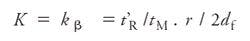
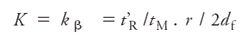
where K is the distribution constant. While the phase ratio (β) of the two columns is normally not much different, the short length and high carrier flow rate leads to very low retention times of a few seconds on the ²D columns.

Time, Peak Capacity, and Speed

In much of the GC×GC literature, total analysis time has not been of critical concern. Generally, because we achieve such a high peak capacity, and very many peaks for GC×GC, most researchers have been interested in displaying the full compositional heterogeneity of a sample, with as many resolved peaks as possible. Indeed, demonstrating the sheer complexity of many samples has been a very attractive goal for researchers. The peak generation potential per minute for GC×GC is perhaps 5–10 times greater than that of a single column analysis.

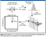
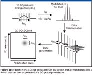
Figure 2

However, with this available separation power, it is possible to sacrifice some of this power to produce a much faster analysis, but with still much more separation than a single column. This contrasts with the usual objective of fast GC — which is to have a faster analysis while preserving about the same separation power of the analysis.

Thus, chromatographers are familiar with the idea of scaling a GC run to reduced dimensions, which gives faster conditions. Typically, we use a shorter, narrower bore column, with faster carrier flow rate (with hydrogen) and usually higher temperature program rate to produce an equivalent separation in a fraction of the time. The Agilent method translation software (Agilent Technologies, Santa Clara, California) is a convenient tool to assist in this choice. Conceptually, the same scaling can be applied to GC×GC; however, this is not often done. We tend to accept a 45–60 min analysis.

Let us walk through the process of making a GC×GC run faster.

Because the total analysis time is controlled largely by the first column time, we have to make this dimension faster — shorter column, higher carrier flow, thinner film, and higher temperature program rate are the options. At the moment, let us just say that the ¹D column elution is faster. Clearly, this is easy to achieve, although a higher carrier pressure risks exceeding the instrument capability.

This now requires us to consider sampling of the ¹D peaks. The ¹D peak width (1w_b) will be smaller. We can either sample fewer times (a smaller modulation ratio, M_R) or sample faster (smaller modulation period, P_M), or both. Small M_R means we can undersample the ¹D peak, and this can lead to losing some of the resolution that has been achieved on the first column. However, the extent to which this compromises a separation still must be quantified. Looking at Figure 2, if the first peak is very narrow, then maybe only one modulation pulse will be attained, and it is possible that neighboring peaks that are resolved on the first column will be now be captured into the same modulation event, and this can degrade the total resolution. If we do not reduce the modulation period (that is, let P_M ~ 5 s), then a fast analysis with 1w_b = 2 s will lead to M_R ~ 0.4. It is most likely that no GC×GC reports have used such a small M_R setting. So, the best option is to speed up both the chromatography and the P_M. Let P_M ~ 2 s, then M_R ~ 1. This means we can achieve about one or two modulations per peak. Likewise, with P_M ~ 1 s, then M_R ~ 2. Or if peaks are narrower (1 s), M_R will be back to ~1. Clearly, speed of all parts of the process is critical, and we place considerable demands on the system if we want to choose faster analysis.

Case Study 1: Fast GC×GC

The previous arguments have ramifications on how fast the mechanical operation of modulation can give such a fast peak sampling. In the most commonly used methods of cryogenic modulation, which derive from the early research of this group (1–3) from about 1995, the modulation zone must be cycled through effective cooling, then heating, to efficiently trap and then release solute from the modulation interface. While we have achieved such a P_M of 1 s (4) recently, with a 35 °C/min temperature program rate and 5-min analysis time (for a sample conventionally requiring 30–45 min), faster operation was not considered, because the maximum practical oven program rate had been reached. However, it was found essentially that the 2-D separation space usage was not much different to that in the slower run — we might say that effective method translation was realized. While this shows that we can achieve much faster analysis, the study was not extended to validation of the approach.

Case Study 2: Thermally labile natural products

The analysis of some natural products can be subject to temperature limitations — too high a temperature can lead to compound degradation. Recently, we have studied analysis of natural pyrethrums. It is imperative that temperature not exceed about 200 °C. On a conventional column length, elution temperatures of about 250 °C were found. To some, the obvious solution would have been to try HPLC. However, faster GC×GC can achieve the desired elution condition, with all the inherent benefits of using a GC method. We chose to use a short ¹D column, with on-column injection, and high carrier flow rates of as much as 8 mL/min. Elution temperatures below 200 °C were obtained, but there are complications with the analysis of natural extracts. There are coextracted interferences that lead to poor ability to quantify components with flame ionization detection (FID). However, we reasoned that GC×GC would win back some separation power lost on the first column. But low temperature elution leads to excessively long retentions on the second column. We calculated that k3 values of about 150 were obtained. This increases the retention time excessively, which would mean we would have to use long P_M settings if we did not want wrap-around. So, we chose to use a very short 2-D column with an effective length of about 15 cm. The result was that we could elute target compounds at low temperature, get adequate resolution of matrix interferences by using the ²D column, and quantify the pyrethrums (5).

Case Study 3: Use of low polarity/polar or polar/low-polarity column sets

A further method variation that is becoming much more prevalent is the use of an "inverted phase geometry" column set. Early work essentially used a nonpolar/polar set. This combination was considered the most orthogonal; because the first column separation mechanism is largely by boiling point, which means overlapping peaks have similar boiling points. When they pass to the ²D column, they will then be separated based upon polar interactions. Clearly, this is a very logical approach. Figure 3a illustrates this, where compounds 1 and 2 represent two species with similar boiling points, but 2 is more polar than 1~ likewise 5 is more polar than 4. Peaks 6–10 represent some sort of homologous series and so have incremented boiling points but similar polarities. As successive homologs are eluted later, they have reduced retention on the ²D column (²t_R), which is due to the higher oven temperature. Now, let us switch the column polarities. Figure 3b attempts to display the altered column set selectivities for this hypothetical mixture. Because the nonpolar compound 1 does not favor retention by the polar ¹D column, it now is eluted earlier than 2 on the ¹D column — 2 is more polar and so is retained longer. Because 1 now enters the ²D column at a reduced temperature, it is retained strongly in the nonpolar phase. We can see, though, that the polar compound is retained poorly by the nonpolar phase, and is eluted from the ²D column with low ²t_R. Peaks 4 and 5 can be argued in similar fashion. The moderate polarity suite 6–10 are retained now later than solute 3, but probably still show a reducing ²t_R trend across the series. The observation of the trend in retention for compounds 6–10 is linked to what we term "structure" within the GC×GC plot, where related compounds often are located along a readily identifiable retention line within the 2-D space. This plot and the fingerprint presentation of a total sample composition are two valuable attributes of GC×GC that are not extracted so readily from single-column analysis. The predictive power of GC×GC has yet to be delineated fully, but we predict that while peak 7 in Figure 3a will overlap peak 3 on the ¹D column, its separation from 3 is compete on the ²D column, and also its relationship to the series 6–10 is unmistakable.

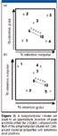
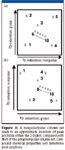
Figure 3

So, we now have a completely different — we might say complementary — strategy for the separation of a mixture. Not only a choice of which polar and nonpolar column phases, but in which order they should be placed. If the polar/nonpolar set does not conform to easy definition or identification of its "orthogonality" principle, this does not detract from its use for enhanced separation. The "clean" boiling point/polarity mechanism of the nonpolar/polar set most probably now becomes (polar + boiling point) mechanism on the first column with (boiling point + polarity) mechanism on the second for a polar/nonpolar set. A more rigorous understanding of the subtleties of such separations must be developed. Marriott and Ryan (6) sought to establish better appreciation of the interplay of polarity on the 2-D presentation by systematically altering the polarity of the ¹D column though coupling together columns of high and low polarity. The relative positions of peaks of different boiling points and polarity will change in response to the net column polarity, which affects elution temperature and alters retention on the ²D column.

As examples of the different results achieved following the inverted phase arrangement, the following should be instructive.

Petrochemical samples: A nonpolar/polar set produces a retention order on the second column of alkanes < cyclic alkanes < olefins < aromatics. The compressed separation of the first two classes, which contains many isomers, gives a reduced resolution for these compounds. Aromatics are well resolved. By using a polar/nonpolar set, the nonpolar compounds are retained more strongly now on the ²D column and have greater resolution. The aromatics are little retained, so tend to be less well resolved than before. Figure 4 compares the two column sets for an oil sample. In Figure 4a, the nonpolar compounds are well spread over the upper part of the 2-D plot, whereas in Figure 4b they are retained poorly and are eluted almost as an apparent unresolved band at the lower part of the plot.

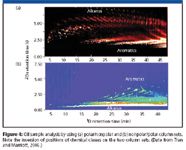
Figure 4

Coffee volatiles: The headspace of coffee contains many polar compounds, such as pyrazines and pyridines. While the aroma of coffee is easily recognizable, and we might think that it therefore comprises compounds in high abundance, generally we have a very complex mixture with no particular compound dominating. If we use a nonpolar ¹D column (Figure 5a), polar compounds are eluted at relatively low temperature, and so when they are introduced to the polar ²D column, they are retained strongly. This causes significant bunching of many compounds at low retention in the 2-D plot (7). Using a polar/nonpolar strategy, the polar solutes are better retained so are drawn out along the ¹D column, and then are retained not too strongly on the ²D column. This approach gives a much better 2-D analysis, as shown in Figure 5b.

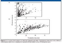
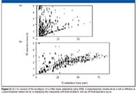
Figure 5

Fatty acid methyl esters (FAME): There are now good GC×GC methods for FAME based upon nonpolar/polar column sets (8,9). The first column choice is not consistent with the usual choice of column for 1-D GC of FAME, which tend to be high % cyano-propyl siloxane phases. On nonpolar phases, there tends to be much less separation within a given carbon number group of FAME (with more highly unsaturated FAME eluted earlier, and the saturated FAME last among the group), compared with that on the cyano-propyl phase (which inverts the elution order and the saturated FAME is eluted first). However, having a polar ²D column gives a very selective separation based upon degree of unsaturation and geometric structure of the FAME. Figure 6 illustrates a reference FAME sample showing that increased degree of unsaturation leads to later ²D elution for this column set. The expanded C₁₈–C₂₀ region provides a demonstration of how molecular structure differences leads to chromatographic "retention structure" differences in the 2-D plane. This retention structure can be likened to, and treated in much the same way as, a fingerprint, and the pattern should be consistent from one FAME group to another (for example, for C-18 and C-20 FAME groups). This technique promises to be a powerful identification tool as trends and relationships are established for such patterns. A column set with a nonpolar ²D column tends to align all the FAME into almost an exponential line within the 2-D space, which suggests the retentions are correlated somewhat, and little differentiation is achieved.

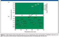
Figure 6

Summary

GC×GC is rapidly being established as a unique and valuable tool for volatile chemical analysis. Its capabilities extend those of single-column GC in a range of unique ways, and so new information is provided to the analyst. By challenging GC×GC methods in new application areas, and also exploring different ways to implement GC×GC, there is now a suite of knowledge being accumulated that offers compelling evidence that GC×GC is here to stay.

"Column Watch" Editor Ronald E. Majors is business development manager, Consumables and Accessories Business Unit, Agilent Technologies, Wilmington, Delaware, and is a member of LCGC's editorial advisory board. Direct correspondence about this column to "Sample Prep Perspectives," LCGC, Woodbridge Corporate Plaza, 485 Route 1 South, Building F, First Floor, Iselin, NJ 08830, e-mail lcgcedit@lcgcmag.com

Ronald E. Majors

Philip Marriott (PhD) is Professor of Separation Science at RMIT University, and Deputy Director of the Australian Centre for Research on Separation Science (ACROSS). He has held appointments at the University of Bristol and in Singapore. His major research interests are in applications and fundamental understanding of multidimensional and comprehensive 2D GC, mass spectrometry and capillary electrophoresis applications.

Paul Morrison is technical research scientist in the ACROSS group at RMIT University. He provides technical support and systems development for innovative implementation of multidimensional methods in GC, and has interests across a wide range of separation methodologies.

References

(1) P.J. Marriott and R.M. Kinghorn, Anal Chem. 69, 2582–2588 (1997).

(2) P.J. Marriott and R.M. Kinghorn, J. High Resol. Chromatogr. 19, 403–408 (1996).

(3) R. Kinghorn, P. Marriott, and P. Dawes, J. High Resol. Chromatogr. 23, 245–252 (2000).

(4) S. Bieri and P.J. Marriott, unpublished results (2006).

(5) J. Harynuk and P.J. Marriott, Anal. Chem. 78, 2028–2034 (2006).

(6) D. Ryan, P. Morrison, and P.J. Marriott, J. Chromatogr., A 1071, 47–53 (2005).

(7) D. Ryan, P. Shellie, P. Tranchida, A. Casilli, L. Mondello, and P. Marriott, J. Chromatogr., A 1054, 57–65 (2004).

(8) R.J. Western, S.S.G. Lau, P.J. Marriott, and P.D. Nichols, Lipids 37, 715–724 (2002).

(9) L. Mondello, A. Casilli, P.Q. Tranchida, P. Dugo, and G. Dugo, J. Chromatogr., A 1019, 187–196 (2003).