The Gradient Delay Volume, Part II: Practice – Effects on Method Transfer

The gradient delay volume is one of the most important, yet least understood, parameters that affect how gradient elution separations in liquid chromatography (LC) work. This parameter has implications for method development and method transfer during the lifecycle of an LC method. In this installment, I illustrate the impact of different gradient delay volumes when transferring a method between instruments and discuss some strategies that can be used to mitigate these challenges.

In my interactions with people learning about various aspects of liquid chromatography (LC), I find that the concept of the “gradient delay volume” (GDV) is one of the most difficult ideas to grasp and apply in practice. I find this to be the case both for true beginners—students who are just learning the basics of LC—and for more experienced scientists who have always dealt with GDV, knowingly or unknowingly, but are perhaps having to think about its impact on their work in new ways. The GDV concept has been important since the first times LC separations involving changes in the mobile phase composition—now known as “gradient elution” separations—were made during an analysis. However, given the various ways that GDV can impact the practice of LC, and that we continue to see changes in commercial instrumentation that affect the way we interact and think about GDV, I think a dive into the details is warranted here. In last month’s installment of “LC Troubleshooting,” I reviewed the basic elements of the GDV concept and discussed how we understand that GDV affects characteristics of LC separations from a theoretical point of view. In this month’s installment, I discuss the implications of these ideas, with an emphasis on how the differences in GDVs between instruments can impact how a particular method will function on said instruments.

The GDV is commonly referred to by others as the “gradient dwell volume,” or sometimes just “dwell volume.” I prefer the inclusion of “gradient” to make it clear what we are talking about, and I prefer “delay” over “dwell” because “delay” communicates one of the most important impacts of GDV—that it delays the arrival of a programmed change in the mobile phase composition at the column inlet. Nevertheless, from my point of view, “gradient delay volume” and “gradient dwell volume” refer to the same thing.

In this two-part series on GDV, we discuss details in a way that assumes we are talking about the reversed-phase (RP) mode of LC. However, most of the discussed ideas are applicable to other modes of LC separation, such as hydrophilic-interaction chromatography (HILIC) and ion-exchange chromatography (IEC).

Finally, readers interested in learning more about GDV will not have a hard time finding good resources, and they are encouraged to consult them. A short list includes several articles in the LCGC magazine, and the book by Snyder and Dolan that is focused entirely on gradient elution LC (1). The relatively recent books edited by Stavros Kromidas have rich sections written by major instrument vendors that explain in some detail the software- and hardware-oriented approaches they have taken to effectively achieve variable GDV in their instruments (2,3). Searching the LC Troubleshooting Bible website (https://lctsbible.com/) for the keyword “dwell volume” will immediately return about a dozen articles from the last 20 years.

Potential Impacts of Gradient Delay Volume on Transferability

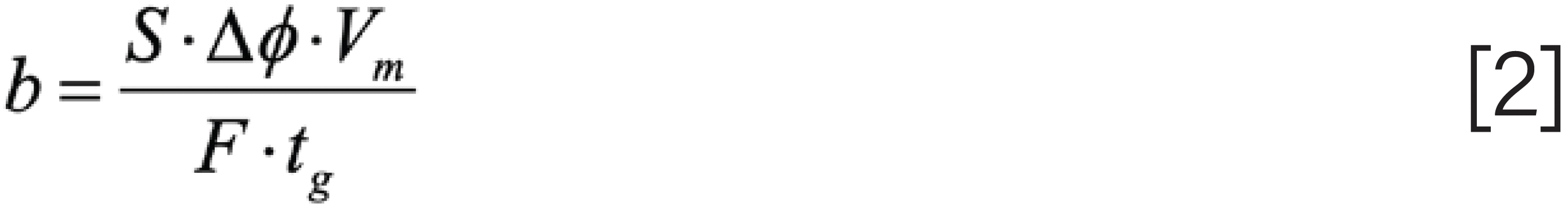
In last month’s installment, I reviewed the essential elements of the theory of gradient elution with an emphasis on the primary variables that control analyte retention time, explaining how GDV influences these relationships. I repeat two of the most important relationships here for convenience. Equation 1 shows the relationship between the retention time (t_r) and the column dead volume (V_m), mobile phase composition used as the starting point in the gradient (ϕ_i), change in mobile phase composition during the gradient (Δϕ), GDV (V_d), and the flow rate (F) (4). The parameter b is known as the gradient slope, given by Equation 2, where t_g is the gradient time. Finally, k_i is the retention factor of the analyte in the mobile phase used as the starting point in the gradient (that is, ϕ_i). The parameter S is analyte-specific, and depends on the mobile- and stationary-phase chemistries and temperature, and it is obtained from the slope of a ln(k) vs. mobile phase composition (ϕ, on a 0–1 scale, where 0 represents pure weak solvent, and 1 represents pure strong solvent). Note that Equation 1 assumes that the plot of ln(k) vs. ϕ is linear (that is, we are using the Linear Solvent Strength Theory here).

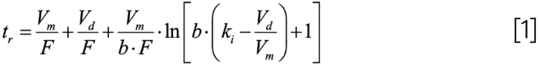
The challenges we face with the transferability of gradient elution methods arise from the relationship between the GDV (V_d) and other variables in Equation 1. V_d appears both inside and outside of the log term, and also very importantly, in the numerator of the ratio V_d/V_m.

Impact of GDV on Transfer of a Method from One LC System to the Next

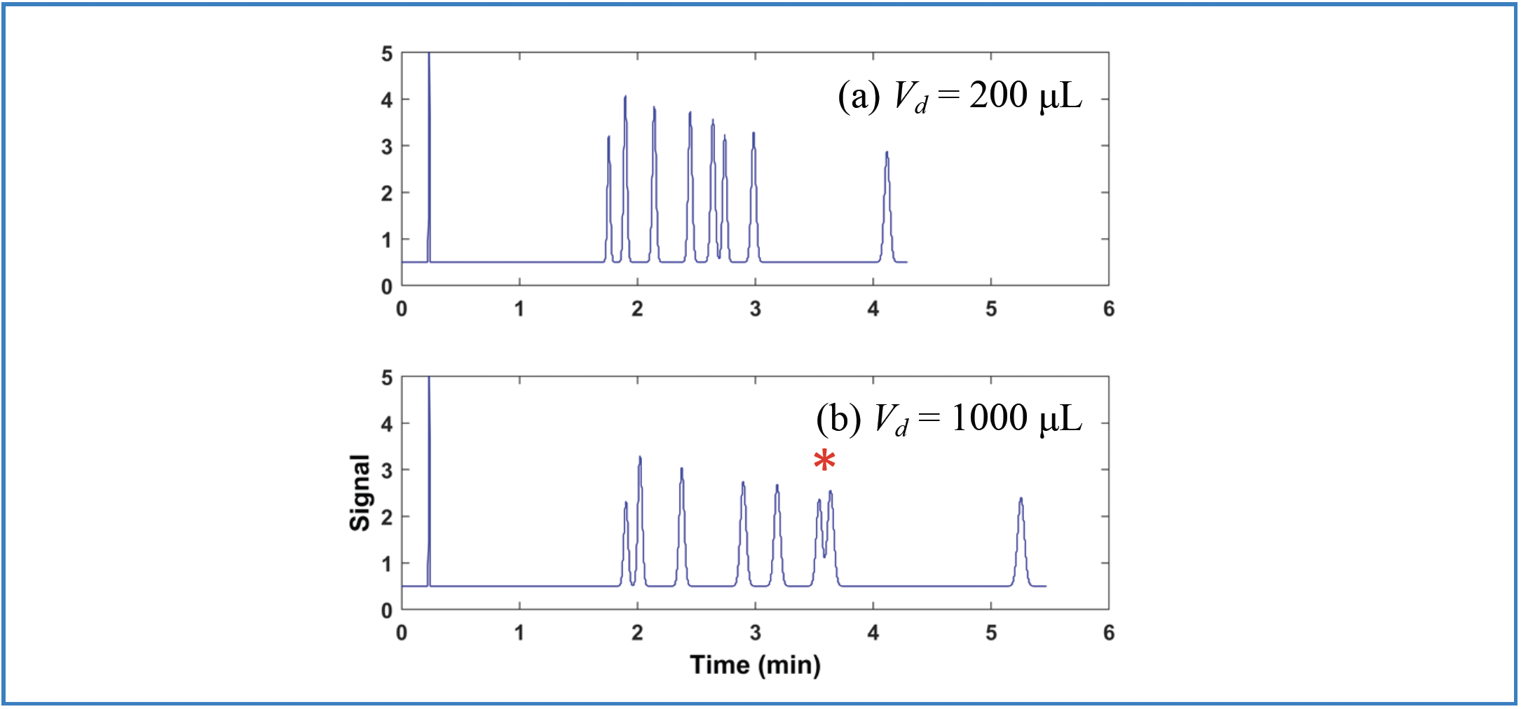
In contemporary LC practice, it is quite common for a method to be developed in one laboratory, but applied for many years in one or more other laboratories—sometimes on different continents, and sometimes in the laboratories of different companies. In these situations, it is inevitable that, at least at some point in the lifecycle of the method, the different LC systems used for development and application of the method will be from different manufacturers, with different designs and GDVs. This can lead to outcomes like those illustrated in Figures 1 and 2. In the scenario illustrated in Figure 1, a method has been developed using an instrument with a GDV of 200 μL, but it was applied using an instrument with a GDV of 1000 μL. Whereas the mixture of eight components is nicely resolved using the development system (Figure 1a), the resolution for the critical pair when applying the method is only approximately 1.0 (Figure 1b), which is clearly a major problem.

FIGURE 1: (a) V_d = 200 μL and (b) V_d = 1000 μL. Comparison of separations for a mixture of small molecules obtained on systems with different GDVs. Chromatograms are simulated (www.multidlc.org/hplcsim) using the following parameters: Stationary phase, C18; Column dimensions, 50 mm × 2.1 mm i.d. (1.8 μm particle size); Flow rate, 0.4 mL/min.; Temperature, 40 °C; Gradient elution from 20–45% B from 0–6 min.; (a) solvent, water; (b) solvent, acetonitrile. The red asterisk indicates ethylparaben and nitrobenzene are coeluted. Other compounds are uracil, methylparaben, 3-phenylpropanol, benzonitrile, p chlorophenol, acetophenone, and propiophenone.

FIGURE 2: (a) V_d = 1000 μL and (b) V_d = 200 μL. Comparison of chromatograms obtained on systems with different GDVs, but with a method that had been developed using the system with the larger GDV. Conditions are the same as in Figure 1, except that the gradient was 15 40% B from 0–6.5 min.

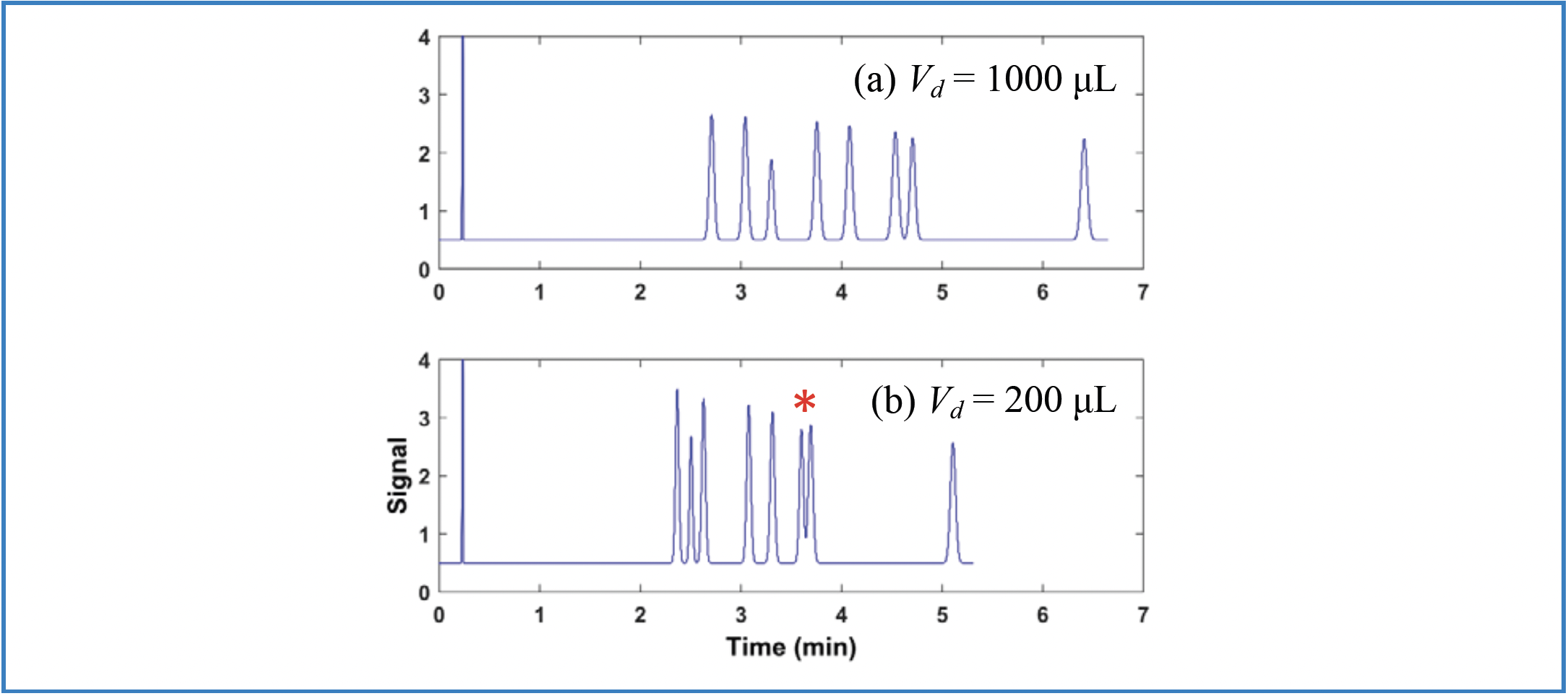
Figure 2 illustrates the opposite situation, where the method is developed using a LC system with a GDV of 1000 μL, and then applied using a system with a GDV of 200 μL. In this case, the conditions were adjusted to obtain a baseline resolution of the sample using the development system, even though the GDV is large at 1000 μL (Figure 2a), and the separation is adequate. However, when this method is run on the system with the lower GDV of 200 μL, again we see coelution, in this case for the same critical pair (ethylparaben and nitrobenzene) as in Figure 1b.

Impact of GDV on Transfer of a Method from One Column to the Next

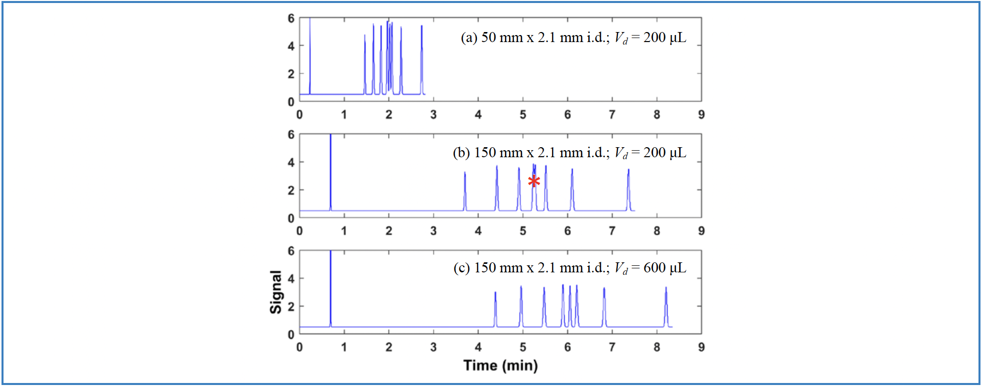
It is also common during method development to do an initial screening of conditions (mobile and/or stationary phases) using a short column, and then move to a longer column for more efficiency and resolution once a small number of candidate conditions have been identified. Ideally, the columns of different lengths would have exactly the same selectivity so that the conditions worked out with the short column can be transferred to the longer column without any unexpected changes in selectivity. However, even if the columns do have exactly the same selectivity, unexpected decreases in resolution can occur when moving to the longer column because of the impact of the GDV on retention time. Panels A and B of Figure 3 show an example of this scenario. In Figure 3a, the mixture is nicely resolved in under 3 min using a system with a GDV of 200 μL and a 50 mm × 2.1 mm i.d. column. Now, when we move to a longer column, we should scale the gradient time accordingly if we want to realize the same selectivity observed with the short column. However, we see in Figure 3b that when the gradient time is tripled inline with the tripling of the column length, we have a serious coelution of p-chlorophenol and ethylparaben in the middle of the chromatogram. This coelution occurs because the ratio V_d/V_m inside the log term in Equation 1 changes if we change the column dimensions without changing the GDV. As soon as we increase the GDV by a factor of three so that the ratio V_d/V_m stays constant, we see in Figure 3c that the same selectivity is realized as in Figure 3a, but with increased resolution because the longer column provides more efficiency (that is, plate number). Therefore, the important takeaway here is that when changing column dimensions, we should be sure to change two other variables if we want to maintain the selectivity with the new column: 1) the gradient time should be adjusted in proportion to the ratio of the column volumes (more generally, the gradient volume should be adjusted; this is critically important if the flow rate is also changed); and 2) the GDV should be adjusted so that the ratio V_d/V_m stays constant (5).

FIGURE 3: Illustration of the interactions between column dimensions and GDV, and their effects on resolution. Conditions are the same as in Figure 1, with the following exceptions: (a) gradient is 20–60% B in 0–3 min; (b,c) gradient is 20–60% B in 0–9 min. The red asterisk indicates the coelution of p-chlorophenol and ethylparaben.

Solutions to the Transferability Challenge

The challenge encountered in the second scenario discussed above where a method is developed using a system with a larger GDV and applied using a system with a smaller GDV (see Figure 2) is easier to address than the reverse scenario (see Figure 1). This is because the solution involves making the instrument with the smaller GDV behave as though it has a larger GDV. Instrument manufacturers have implemented a variety of creative technological solutions in recent years to address this, which involve software- or hardware-oriented solutions, or both. For example, a Chromatography Data System (CDS) could “know” that one way to increase the effective GDV is to simply program an isocratic hold into the beginning of the solvent gradient program that is executed by the pump. This would be an example of a software-oriented solution that does not require any physical changes to the instrument hardware. In this case, one could configure the instrument to always behave as if it had a specified effective GDV that is larger than the physical, and apply that behavior to all methods, rather than having to program the isocratic hold into each method. On the other hand, the physical configuration and behavior of the instrument can also be changed to adjust the effective GDV. For example, pieces of tubing with known volumes can be mounted onto a switching valve so they can be introduced into the flow path between the pump and column under software control. Alternatively, the effective volumes associated with components in pump heads and sampler syringes can also be adjusted by changing the positions of pistons in those devices. Again, all the examples mentioned here have been implemented by manufacturers in commercial instruments. Readers interested in learning more about these possibilities are encouraged to reach out to salespersons for the instruments they have in their laboratories.

Solutions to Consider When Moving to a System with a Larger GDV

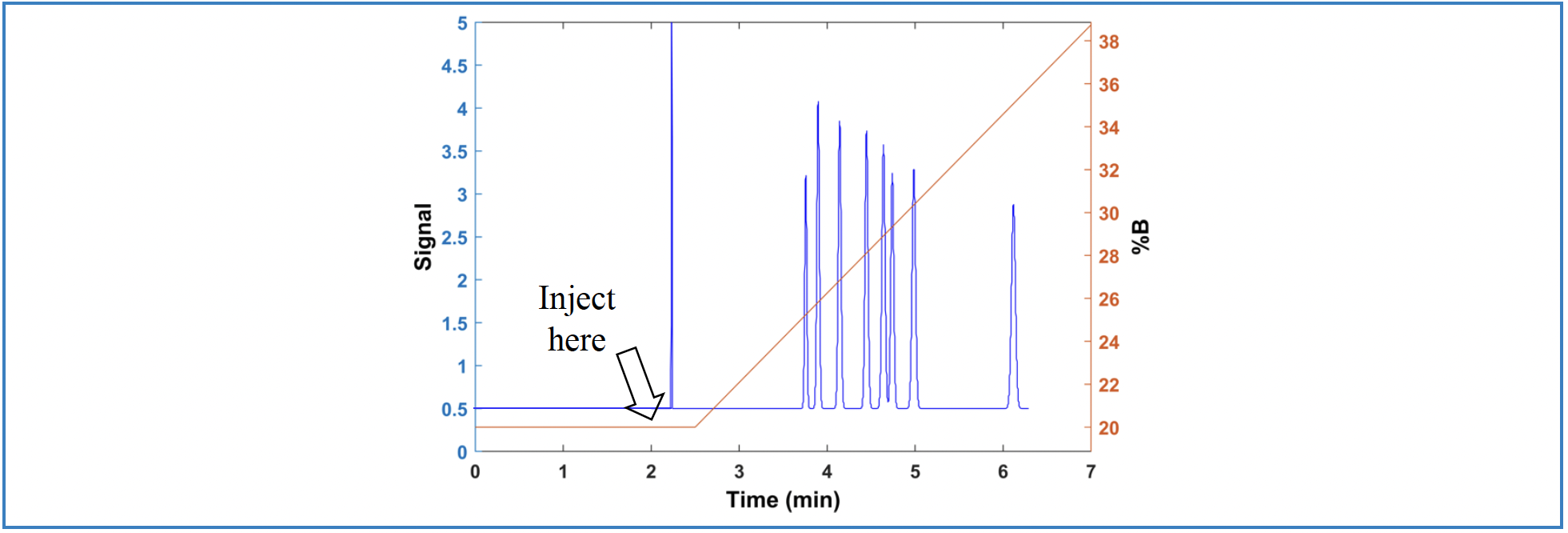
There are two approaches that have been commonly used to address the challenge described in the first scenario illustrated in Figure 1 (6). The first is that the sample injection can be delayed relative to the start of the method (and thus, the start of the “clock” against which the gradient delay time is calculated). In this case, the physical GDV is not changed, but the effective GDV is reduced by the product of the injection delay time and the flow rate. This approach is illustrated in Figure 4. Most modern LC instruments support time-delayed injections, and one of the advantages of this approach is that the degree of adjustment is highly variable and software-controlled.

FIGURE 4: Simulated chromatogram for a system with GDV of 1000 μL, but with a delayed injection such that the effective GDV is 200 μL. Other conditions are the same as in Figure 1a.

The second, and more widely implemented approach, is to deliberately add an isocratic hold to the solvent gradient program early on in method development, even if the physical GDV is rather small. The idea here is that if the added isocratic hold is chosen to be as large (in volume terms; V_d = t_d*F) as the GDV of any instrument the method could possibly be transferred to, then the method developed on the system with a low physical GDV can be transferred to any instrument with a large physical GDV. In this case, adjustment of the method would principally involve adjusting the length of the isocratic hold to account for the difference between the GDVs of the two instruments (that is, the development instrument and the application instrument). The upside of this approach is that it can be very effective. The downside is that the GDVs of instruments the method might be transferred to in the future have to be anticipated early on in the method development process.

Other Practical Factors

Two other practical factors that deserve mention here are the “rounding” of solvent gradient profiles, and the effect of pressure on GDV. In this installment, I have focused on the gradient delay volume and its impacts on retention, selectivity, and resolution. The volume associated with the fluidic components between the pump and the column is indeed the primary determinant of these effects. However, the geometries of these components (for example, lengths, diameters, and shapes) influence the “rounding” of the solvent composition profile that actually arrives at the column inlet. This is because of axial dispersion of the mobile phase components, which in turn is influenced by the geometries of the fluidic components. Although these effects are secondary, they can be quite important in some situations. Readers interested in learning more about this aspect are referred to the literature on the topic (7,8).

Finally, some older designs of LC pumps relied on “pulse dampeners” to smooth out pressure fluctuations in the mobile phase delivered by the pump. These dampeners involved compressible fluids whose volumes depended on pressure, resulting in a significant dependence of the observed GDV on pressure. Most modern LC pumps do not rely on such dampeners, but this is something to be aware of when working with older instrumentation.

Summary

In this installment of “LC Troubleshooting,” I’ve discussed the impact of gradient delay volume (GDV) on the transferability of gradient elution methods between instruments with different GDVs, and with columns of different dimensions. We can run into trouble moving in both directions—that is, moving from a system with a small GDV to a system with a larger GDV, or vice versa. Fortunately, these challenges can be mitigated using software- or hardware-based approaches to change the effective GDV of an instrument available in most modern LC instruments. Transferring methods from modern instruments to older ones with much larger GDVs can be challenging, but is facilitated by building in method features early in the development process that anticipate the need to transfer the method later on in the method lifecycle. Understanding the theoretical influence of GDV on retention, selectivity, and resolution, and the implications of these effects in practice give us a rational means of coping with the GDV during method development and troubleshooting.

References

(1) Snyder, L. R.; Dolan, J. W. High-Performance Gradient Elution: The Practical Application of the Linear-Solvent-Strength Model; John Wiley: Hoboken, NJ, 2007.

(2) Gradient HPLC for Practitioners: RP, LC-MS, Ion Analytics, Biochromatography, SFC, HILIC; Kromidas, S., Ed.; Wiley-VCH: Weinheim, 2019.

(3) Optimization in HPLC: Concepts and Strategies; Kromidas, S., Ed.; Wiley-VCH: Weinheim, 2021.

(4) Schoenmakers, P. J.; Billiet, H. A. H.; Tussen, R.; De Galan, L. Gradient Selection in Reversed-Phase Liquid Chromatography. J. Chromatogr. A 1978, 149, 519–537. DOI: 10.1016/S0021-9673(00)81008-0

(5) Schellinger, A. P.; Carr, P. W. A Practical Approach to Transferring Linear Gradient Elution Methods. J. Chromatogr. A 2005, 1077 (2), 110–119. DOI: 10.1016/j.chroma.2005.04.088

(6) Snyder, L. R.; Dolan, J. W. Chapter 5: Separation Artifacts and Troubleshooting. In High-Performance Gradient Elution: The Practical Application of the Linear-Solvent-Strength Model; John Wiley: Hoboken, NJ, 2007; pp 153–224.

(7) Magee, M. H.; Manulik, J. C.; Barnes, B. B.; Abate-Pella, D.; Hewitt, J. T.; Boswell, P. G. “Measure Your Gradient”: A New Way to Measure Gradients in High Performance Liquid Chromatography by Mass Spectrometric or Absorbance Detection. J. Chromatogr. A 2014, 1369, 73–82. DOI: 10.1016/j.chroma.2014.09.084

(8) Bos, T. S.; Niezen, L. E.; den Uijl, M. J.; et al. Reducing the Influence of Geometry-Induced Gradient Deformation in Liquid Chromatographic Retention Modelling. J. Chromatogr. A 2021, 1635, 461714. DOI: 10.1016/j.chroma.2020.461714

ABOUT THE AUTHOR

Dwight R. Stoll is the editor of “LC Troubleshooting.” Stoll is a professor and the co-chair of chemistry at Gustavus Adolphus College in St. Peter, Minnesota. His primary research focus is on the development of 2D-LC for both targeted and untargeted analyses. He has authored or coauthored more than 75 peer-reviewed publications and four book chapters in separation science and more than 100 conference presentations. He is also a member of LCGC’s editorial advisory board.