Treat it Like a Circuit, Part I: Comparison of Concepts from Electronics to Flow in LC Systems

The analogy that electrons flowing in wires is like water flowing through a tube can be remarkably effective for teaching and learning about fluid flow in liquid chromatography (LC) systems. In this installment, we will go over the basics of this analogy, as well as explicitly discuss the phenomena observed in the two cases and the physical laws that we can use to rationalize and predict the behavior that we see. In the second installment in this series, we will then use this knowledge to demonstrate how these ideas can be used to troubleshoot problems when they arise in LC systems.

In my interactions with liquid chromatography (LC) users from various backgrounds and levels of training and experience, I observe that perceptions about how flow and pressure “work” in LC systems vary dramatically from one user to the next. In some cases, I see that the fluidics of the LC system are treated as a black box, without any concrete sense for what the driving forces are, which variables are dependent on others, and in what ways. In other cases, I hear people talk about the behavior of the fluidics in ways that are simply incorrect. Neither of these situations is helpful when it comes to troubleshooting a system that has some flow or pressure related problem. In discussing these observations with Jim Grinias, professor of Chemistry at Rowan University, I found that we agree on two points: 1) many LC users would be better troubleshooters if they had a better understanding of how the fluidics of LC systems “work”; and 2) that there is great value in borrowing concepts from electronics that describe the flow of electrical current in circuits to help us understand and predict the flow of liquids in LC systems. Thus, I’ve asked Jim to join me in writing a two-part series focused first on fundamental concepts in Part I, and then the application of those concepts to real problems in LC systems in Part II. — Dwight Stoll

Opening Thoughts

The technical backgrounds of LC users are remarkably diverse. We think this is actually a testament to the incredible flexibility and utility of LC as an analytical technique. Of course, there are LC users who have taken multiple courses in analytical chemistry, and maybe even have an advanced degree in analytical chemistry or chemical engineering. But, there are probably just as many (maybe even more) LC users with no formal training in separation science in their background. For example, most biology degree programs don’t require a course in analytical chemistry, and yet there are many biologists using LC every day, simply because LC is a very powerful tool for answering a variety of biologically-oriented questions—for example, how do the metabolites in my cell line change in response to a chemical stimulus? In our discussions in preparation for this installment, we realized that the average LC user has probably had more exposure to concepts in physics, including electricity and magnetism, than concepts in hydraulics; therein lies at least some of the value in drawing comparisons between the flow of charge in electrical systems, and the flow of fluids in LC systems. If we can leverage knowledge and concepts from prior experiences with electricity and apply them to understand how LC systems work, we will be better prepared to diagnose and resolve problems encountered with LC systems.

Please note that this discussion is framed using terms in a way that is meaningful for practicing chromatographers, and is not intended to be an in-depth treatment found in an electronics textbook or physics lecture. As a result, some field-specific misnomers may occur, but these do not affect the utility of the central idea of treating electronic and fluidic circuits similarly in the context of LC troubleshooting. Readers interested in diving into these topics in more detail are referred to respected texts in the field (1,2).

Definitions, Relationships, and Concepts

In both electrical and fluidic systems, there has to be a driving force that results in the movement of matter from one place to another. In electrical systems, we speak of voltage differences between two points, or voltage drops, that result in the movement of electrical charge (that is, current) between the two points. Similarly, in fluidic systems, we speak of pressure drops that result in the movement of fluid (that is, the molecules that make up the fluid; we simply refer to this as the flow). In both cases, it is instructive to think of matter (electrons or molecules) moving from an area of high potential energy to an area of lower potential energy, and the voltage or pressure drop are ways of quantifying the energy gradients. Once we accept the idea that these drops (voltage or pressure) result in the movement of matter (electrons or molecules), then a number of other useful comparisons can be made between the two systems.

Comments on These Relationships and Their Implications

How to Think About the Unifying Relationship: Proportional vs. Inversely Proportional

Simply writing down the expressions in Table I is one thing. More important is how we think about them and apply them in practice when working with real systems. The magnitude of the flow, whether the flow involves movement of electrons or fluids, is directly proportional to the energy difference. Anything we do to increase the energy difference will immediately result in an increase in the flow (if we don’t change anything else). This relationship is most familiar when thinking about electrical systems where it is usually the voltage drop that is nominally fixed (as in the case of a battery). Here, when we connect a battery to a circuit having a certain resistance, current will flow in the circuit in response to the voltage drop. Since the voltage of the battery is fixed, anything we do to increase or decrease the resistance in the circuit (for example, changing the length of the resistor) will immediately result in a decrease or increase in the current in the circuit.

TABLE I: Comparison of concepts in electrical and fluidic systems

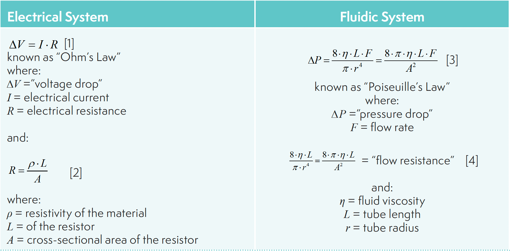
Another way of thinking about this formulation is that an energy difference will result from a certain flow dictated by the operator of the system. Moreover, for a given flow rate, the energy difference that results is dependent on the resistance in the circuit. Anything we do to decrease the resistance in the circuit will immediately result in a decrease in the energy difference if all other variables are held constant in addition to the flow. This relationship is most familiar when thinking about fluidic systems where it is usually the flow that is nominally fixed, as in the case of an LC pump with a user-defined flow rate. Here, when we turn on the pump connected to tubing and other components with a certain flow resistance, we will see the energy difference develop. We refer to this as the pressure drop, which is typically measured at the pump, but this is really a measure of the pressure difference between a measurement point in the pump and atmospheric pressure (typically taken as zero for practical purposes). In this case, since the flow is fixed (as a setting in the pump), anything we do to increase or decrease the resistance in the flow path (for example, changing the length of connecting tubing) will immediately result in a decrease or increase in the measured pressure drop.

Details of (Flow) Resistance

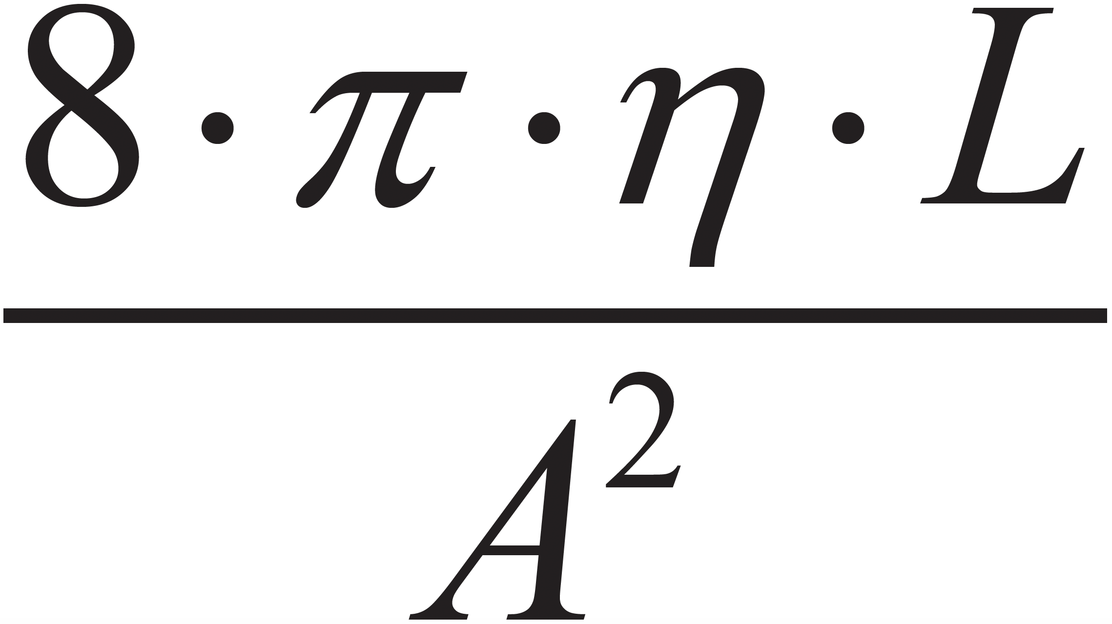
Equations 2 and 4 in Table I provide a more detailed perspective on the factors that dictate resistance to flow in electrical and fluidic systems. Here it is convenient to consider the simplest cases in each system. In the electrical case, we can consider a wire connecting a voltage source to ground, which has a certain length, cross-sectional area, and resistivity (that is, a property of the material the wire is made of). In the fluidic case, we can consider a piece of tubing connecting the outlet of a fluid pump to a waste container open to the atmosphere, where the tubing has a certain length and cross-sectional area associated with the inside, open part of the tube. In the fluidic case, the important material property is the viscosity (think of this as how “thick” the fluid is; peanut butter is very viscous, whereas hexane is not) of the fluid flowing through the tubing. We see that in both cases the resistance is directly proportional to the first power of the length, and the first power of the material property. Making the wire or tube longer or shorter will increase or decrease the resistance. Similarly, changing the material properties such that the resistivity or viscosity increases or decreases will increase or decrease the resistance.

Careful readers will notice that there is an important difference between the resistances in the electrical case (the aforementioned equation 2) and the fluidic case (equation 4, also in Table I), namely that in the former case the resistance is inversely proportional to the first power of the cross-sectional area of the wire, and in the latter case the resistance is inversely proportional to the square of the cross-sectional area of the tube. This difference results from the no-slip boundary condition (that is, the velocity of the fluid is zero at the wall of a tube) that is required in fluidic circuits (3). But, in both cases, increasing or decreasing the diameter of the wire or tube will decrease or increase the resistance.

Behavior of Systems Having Multiple Elements

Analysis of Voltage Drops and Pressure Drops

In real electrical and fluidic systems, there are usually multiple elements (for example, multiple segments of tubing joined together, usually of different lengths and diameters), and we need a way to analyze these systems so that we know what to expect from them, which in turn gives us the ability to recognize when something is wrong. Two invaluable tools used in analysis of electrical circuits are Kirchhoff’s Laws, one for voltage, and one for current. Kirchhoff’s Voltage Law asserts that the sum of the “voltage rises” and “voltage drops” around a loop must be zero. Here, by “loop,” we are referring to a closed electrical circuit. In Figure 1a, we see that both ends of the simple circuit are connected to ground, so this is a closed circuit. Starting from the ground point on the left, we encounter a voltage rise at the battery. Then, when current flows through the electrical resistor R_E1, there is a voltage drop from 5 V by the amount i₁∙R_E1, where i₁ is the amount of current. This same current (that is, i₁ = i₂; see below for more discussion on this point) then flows through the second electrical resistor R_E2 to ground, and the voltage drops further by the amount i₂∙R_E2 to 0 V at ground.

FIGURE 1: Illustration of the application of Kirchhoff’s Voltage Law to (a) a simple electrical system, and (b) by analogy to the pressure rises and drops encountered in an LC (fluidic) system.

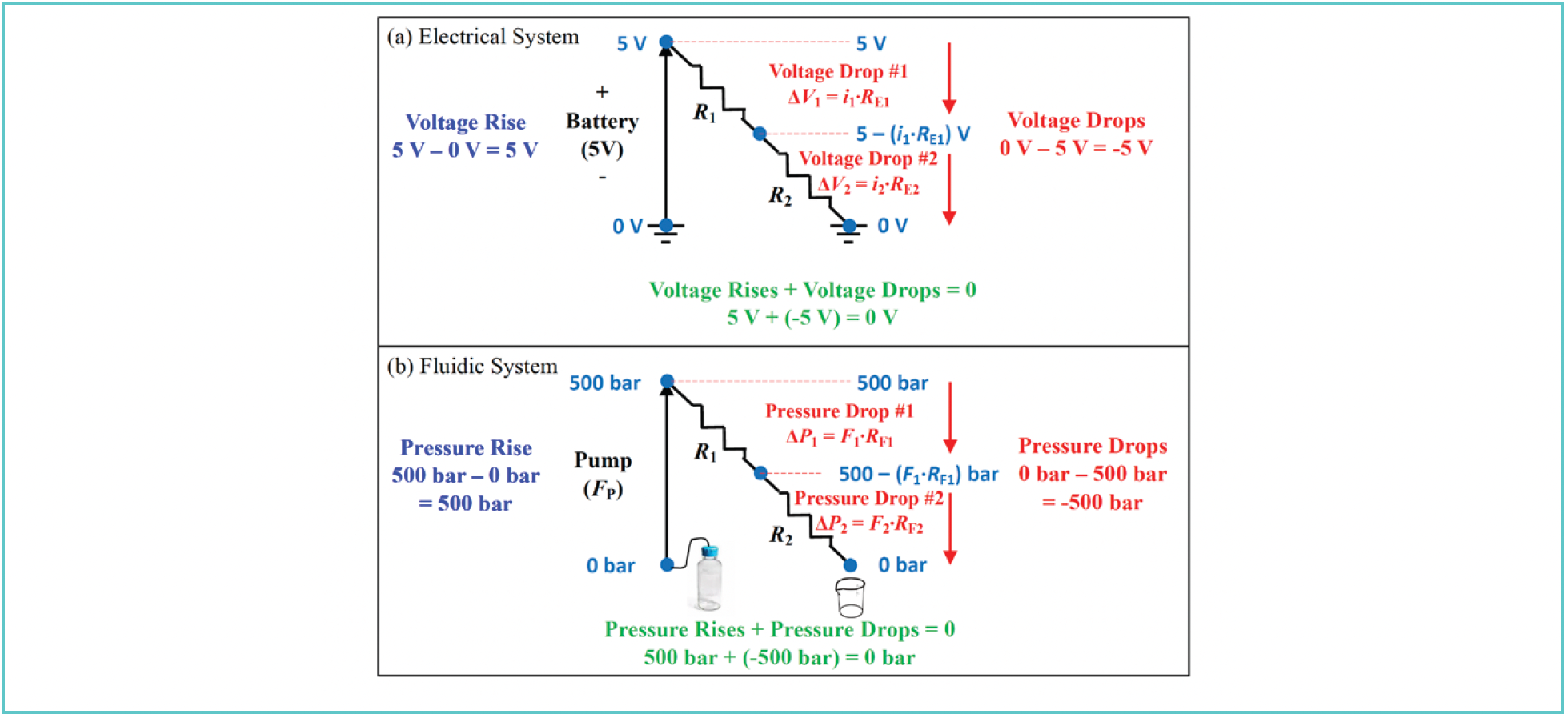
Figure 1b shows the analogous concepts applied to the fluidic system we encounter in an LC instrument. We replace the battery with a pump that produces a user-defined flow rate F_P. As explained above, this flow will result in a pressure measured at the pump. As the mobile phase flows through downstream elements with fluidic resistance the pressure drops first by the amount F₁∙R_F1, and further by the amount F₂∙R_F2 as the mobile phase proceeds toward the waste container that is typically at atmospheric pressure (for our purposes here, this is “fluidic ground”). As in Figure 1a, notice here that F₁ = F₂ (unless there is a leak!). Also note that we have used the shorthand R_F here to indicate fluidic resistance, but this is really

as in equation 4.

What Happens When Elements are Connected?

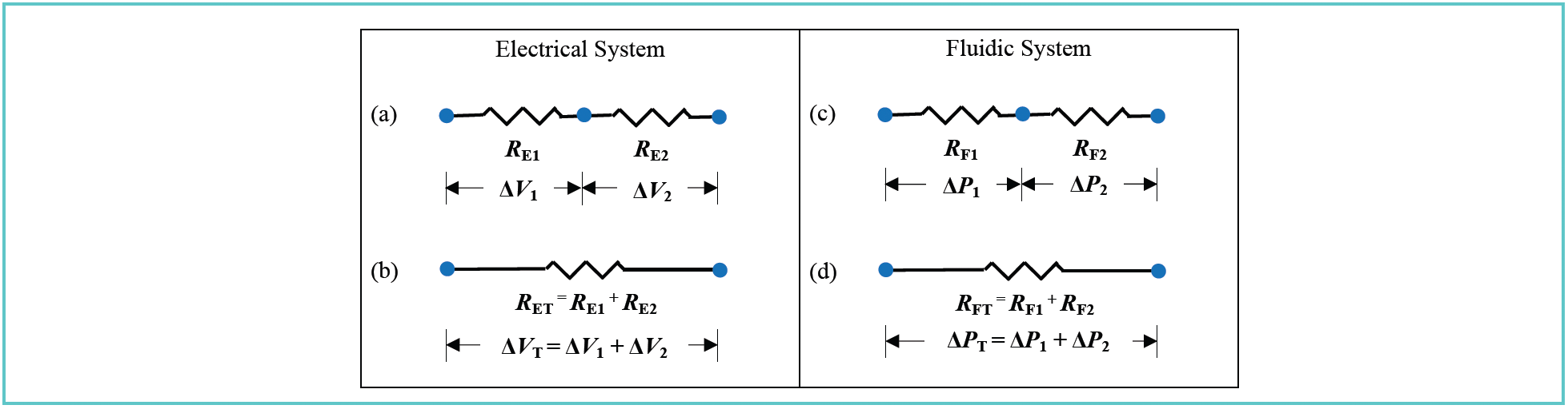
We only concern ourselves here with one situation involving connected components, illustrated in Figure 2, which we refer to as elements connected in series. Elements connected in parallel are also very important in some specific situations in LC, and these will be discussed in next month’s installment. As with the analysis of voltage and pressure drops discussed above, if we understand how systems behave when multiple elements are connected in different ways, we can make predictions about how we expect the systems to behave and observe when things don’t look right. First, Figure 2a shows two electrical resistors connected in series. If we imagine what would be the resistance of a single element needed to replace the two connected resistors (see Figure 2b; in electronics, this is called a Thévenin equivalent), the key idea is that the resistances of two resistors connected in series simply add. Similarly, the voltage drops across each resistor also add such that the voltage drop across the single resistive element (that is, R_ET in Figure 2b) is the sum of the two individual voltage drops ΔV₁ and ΔV₂. Figures 2c and 2d show the comparable diagrams in the fluidic case. We see that the fluidic resistances connected in series add such that the resistance of the single equivalent element (R_FT) is the sum of the two individual resistances R_F1 and R_F2. Also, the pressure drops across the two elements add such that the pressure drop across the single resistive element is the sum of the two individual pressure drops. We will see in next month’s installment that this fact is very useful when troubleshooting pressure problems.

FIGURE 2: Illustration of the relationships between resistances of connected elements in (a,b) electrical systems and (c,d) fluidic systems, as well as the voltage or pressure drops across the elements.

Kirchhoff’s Current Law

Kirchhoff’s Current Law, also known as the junction rule, describes the behavior currents in electrical systems. It is useful to think of it as an expression of the concept of conservation of charge. Specifically, the rule asserts that the sum of the currents into any junction (the blue dots in Figure 3) must be exactly equal to the sum of all currents exiting the junction. That is, all the charge that flows into the junction must flow out of the junction. In Figure 3a, where there is only one current in and one current out, i₁ = i₂. If we add a second conductor connected to the junction on the “out” side carrying a current i₃, then the rule tells us that i₁ = i₂ + i₃. More interesting to chromatographers is the idea that this same kind of rule applies to flows entering and exiting a junction in an LC system. In this case, the fundamental concept in play is the idea of conservation of mass. In Figure 3c, all the molecules of fluid entering the junction must also exit the junction, so that mass is conserved, and F₁ = F₂. This is the most common situation in LC systems. However, if we add a third tube carrying fluid at the flow rate F₃, connected to the outlet side of the junction, then we see that F₁ = F₂ + F₃. We will see that this relationship is particularly useful when making predictions about how a passive flow splitter works, as will be discussed in next month’s installment.

FIGURE 3: Illustration of the application of Kirchhoff’s Current Law to a simple electrical system involving (a,b) components connected at junctions, and (c,d) comparable illustrations of junctions in a fluidic system.

Looking Ahead

Having discussed the essential relationships between flow and pressure in fluidic systems, we are now well positioned to apply these principles to important practical situations encountered in LC systems. In next month’s installment of “LC Troubleshooting,” we will demonstrate how these ideas can be used to systematically troubleshoot common problems related to flow and pressure, and introduce freely available calculation tools that can be used to make predictions about flows and pressures based on inputs of other practical variables such as tubing length and diameter, solvent composition, and temperature. We will also use the ideas discussed here to understand how a passive flow splitter works, and make predictions about split ratio for a given configuration of tubing lengths and diameters used in the splitter. Finally, we will discuss the pressure drop across an LC column containing particles. In this case, equation 3 does not apply, and we need to make some adjustments to the flow-pressure relationship to accurately predict these pressure drops.

Summary

In this installment, we have discussed the idea that concepts from electronics can be used to help understand the relationship between flow and pressure in LC systems. When analyzing electrical systems, Kirchhoff’s Laws concerning voltages and currents can be used to rationalize the behavior of these systems and make predictions about how things are expected to change when a component of the system is adjusted. Analogous relationships can be used when analyzing fluidic systems, which enable us to make predictions about how pressure and flow will change when we make an adjustment to an element of the system, such as changing the diameter of a piece of tubing. In next month’s installment, we will put these relationships and knowledge to work, demonstrating how it all can be used to troubleshoot common problems related to pressure and flow that arise when using LC systems.

References

(1) Horowitz, P.; Hill, W. The Art of Electronics, 3rd ed., 19th printing, Cambridge University Press, 2022.

(2) R.F. Probstein, Physicochemical Hydrodynamics: An Introduction, 2nd ed., Wiley-Interscience, 2003.

(3) Sutera, S. P.; Skalak, R. The History of Poiseuille’s Law, Annu. Rev. Fluid Mech. 1993, 25, 1–20. DOI: 10.1146/annurev.fl.25.010193.000245

ABOUT THE AUTHORS

Dwight R. Stoll is the editor of “LC Troubleshooting.” Stoll is a professor and the co-chair of chemistry at Gustavus Adolphus College in St. Peter, Minnesota. His primary research focus is on the development of 2D-LC for both targeted and untargeted analyses. He has authored or coauthored more than 99 peer-reviewed publications and four book chapters in separation science and more than 150 conference presentations. He is also a member of LCGC’s editorial advisory board.

James P. Grinias is a professor in the department of Chemistry & Biochemistry at Rowan University in Glassboro, New Jersey.