The Gradient Delay Volume, Part I: Theory

The gradient delay volume is arguably one of the most important, yet least appreciated, parameters that affect how gradient elution separations in LC work. This has implications both for method development and for method transfer during the lifecycle of a LC method. In this installment, I will review the concept of gradient delay volume, its physical connection to the LC instrument, and how it can impact method development and separation quality.
In my interactions with people learning about various aspects of LC, I find that the concept of “gradient delay volume” (GDV) is one of the most difficult ideas to grasp and apply in practice. I find this to be the case both for true beginners—students who are just learning the basics of LC—and for more experienced scientists who have always dealt with GDV, knowingly or unknowingly, but are perhaps having to think about its impacts on their work in new ways. The GDV concept has been important since the very first times LC separations involving changes in mobile phase composition were made during an analysis, an approach now known as “gradient elution” separations. However, given the various ways that GDV can impact the practice of LC, and that we continue to see changes in commercial instrumentation that affect the way we interact and think about GDV, I think a dive into the details is warranted here. In this installment of “LC Troubleshooting,” I will review the basic elements of the GDV concept and discuss how we understand that GDV affects characteristics of LC separations from a theoretical point of view. In a subsequent installment, I will discuss the practical implications of these ideas.
A short list of the ways in which the GDV can impact LC separations includes the following:
- Adjusting the GDV, either physically or effectively, through software control, can be used as a variable when optimizing gradient elution separations.
- GDV can be an important parameter affecting the throughput of very fast LC separations.
- Differences between the GDVs of different LC instruments can lead to problems when transferring a method developed on one instrument to a different instrument.
The “gradient delay volume” is commonly referred to by others as the “gradient dwell volume,” or sometimes just “dwell volume.” I prefer the inclusion of “gradient” to make it clear what we are talking about, and I prefer “delay” over “dwell” because “delay” communicates one of the most important impacts of GDV—that it delays the arrival of a programmed change in mobile phase composition at the column inlet. Nevertheless, from my point of view, “gradient delay volume” and “gradient dwell volume” refer to the same thing.
In this two-part series on GDV, I will discuss details in a way that assumes we are talking about the reversed-phase mode of LC. However, most of the ideas that will be discussed are applicable, at least conceptually, to other modes of LC separation, such as HILIC and ion-exchange.
Finally, readers interested in learning more about GDV will not have a hard time finding good resources and are encouraged to consult them. A short list includes several articles in LCGC magazine and the book by Snyder and Dolan, which is focused entirely on gradient elution LC (1). Searching the LC Troubleshooting Bible website (https://lctsbible.com/) for the keyword “dwell volume” will immediately return about a dozen articles from the last 20 years.
What is Gradient Delay Volume?
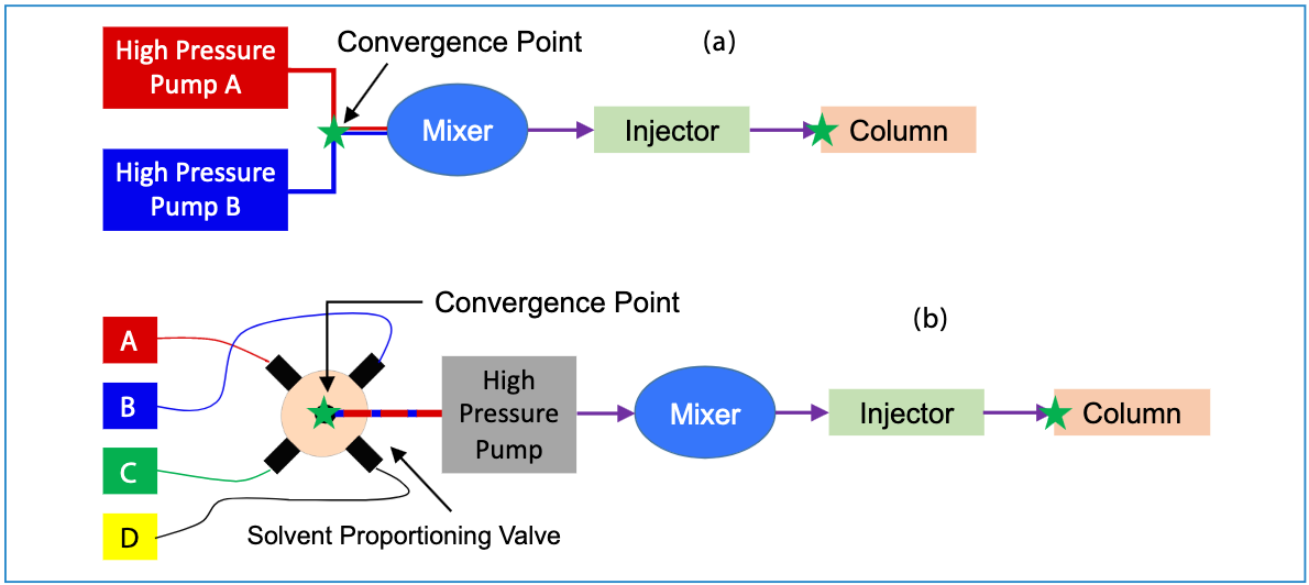
By definition, gradient delay volume is the physical volume that occupies the fluidic path between the point at which two or more solvents are mixed in a LC pump (labeled the “convergence point” in Figure 1) and the column inlet. Figure 1 shows simplified schematic diagrams for the two designs of LC pumps in common use today, which we refer to here as high-pressure mixing and low-pressure mixing designs (see reference [2] for an excellent review of pump designs, as well as a highly educational history of their development). In the case of the high-pressure mixing design shown in Figure 1a, two solvent streams metered by individual high-pressure pumps are brought together at the convergence point, and the combined stream only has to travel through a small mixer and connecting capillaries (and, importantly, the autosampler), before reaching the LC column. In the case of the low-pressure mixing design, the combined solvent flowing out of the convergence point first travels through the high-pressure pump head before moving on to the mixer, sampler, and the column. Typical gradient delay volumes associated only with the pump components (including mixer) are on the order of 50 and 400 µL for modern high- and low-pressure mixing designs, respectively. The gradient delay volumes associated with older models of low-pressure mixing designs were on the order of 1,000 µL. The injector/sampler component of the system can add a little (for example, with low-volume fixed loop injectors) or a lot (for example, with flow through needle designs) of delay volume depending on the design. For example, the additional volume could be on the order of a few microliters for low-volume fixed loop injectors, or as much as a few hundred microliters for a flow through needle design (3).

 high- and (b) low-pressure mixing designs used in LC pumps. The volumes of all components lying between the green stars contribute to the gradient delay volume.")
Figure 1: Simple schematics illustrating the differences between (a) high- and (b) low-pressure mixing designs used in LC pumps. The volumes of all components lying between the green stars contribute to the gradient delay volume.
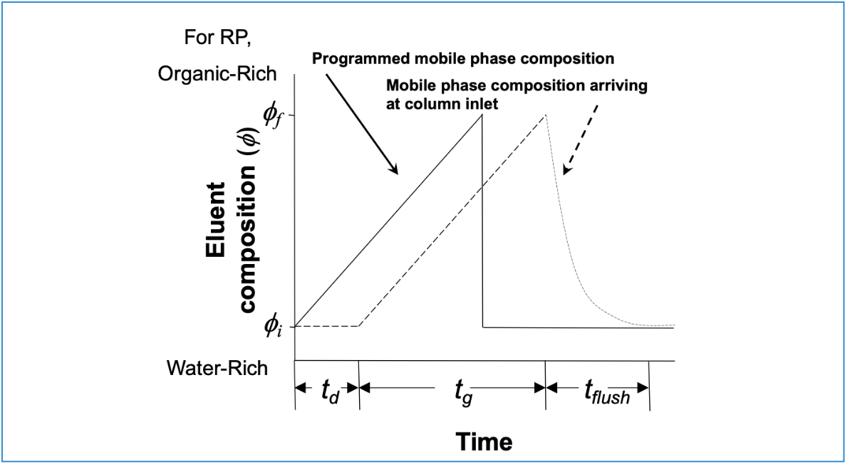
The difference between the mobile phase that we instruct the pump to deliver to the column as part of a gradient elution method, and what is actually delivered to the column, is illustrated in Figure 2. Here, we see that the initial onset of the actual change in mobile phase composition arriving at the column inlet is offset from what we instruct the pump to do by the gradient delay time, td (Vd/F). Then, following completion of the programmed gradient, we see that it takes some time for the strong solvent to be flushed out of the pump components before the actual composition of the mobile phase arriving at the column inlet returns to the composition that will be used as the starting point in the gradient applied in the next analysis. The time required for this flush-out is on the order of 2 × td.

, and the mobile phase composition observed at the column inlet (dashed line). The change in composition is offset in time due to the delay time (td) that results from the time it takes for a change in composition to travel from the solvent convergence point in the pump to the column inlet. Reprinted from reference (4).")
Figure 2: Solvent program used in gradient elution (solid line), and the mobile phase composition observed at the column inlet (dashed line). The change in composition is offset in time due to the delay time (td) that results from the time it takes for a change in composition to travel from the solvent convergence point in the pump to the column inlet. Reprinted from reference (4).
When and Why is the Gradient Delay Volume Important?
Effect on Retention and Selectivity
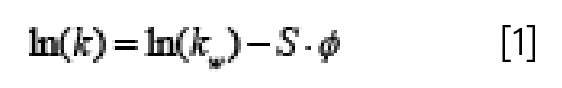
When using gradient elution conditions, it is intuitively evident that any increase in the gradient delay volume will lead to an increase in retention time, simply because it will take longer for the onset of the change in mobile phase composition to reach the column, and thus it will take longer for the composition that actually elutes the compound to reach the column. We can quantify this effect by examining the relationship between retention time and GDV in a preferred retention equation that applies to gradient elution conditions. In the interest of simplicity, we’ll look at the retention equation that comes from linear solvent strength (LSS) theory for reversed-phase LC (1). LSS asserts that the relationship between the logarithm of retention factor and mobile phase composition (ϕ, on a 0–1 scale, where 0 represents pure weak solvent, and 1 represents pure strong solvent) is linear, as shown in equation 1, where ln(kw) is the y-intercept of a plot of ln(k) vs. ϕ, and -S is the slope (see Figure 6 for examples of this type of plot).


In this case, a derivation involving an integration of the distance travelled by the analyte through the column with respect to time yields equation 2, which relates the retention time of the analyte (tr) to ln(kw) and S, the column dead volume (Vm), the mobile phase composition used as the starting point in the gradient (ϕi), the change in mobile phase composition during the gradient (∆ϕ), the GDV (Vd), and the flow rate (F) (5). The parameter b is known as the gradient slope, given by equation 3, where tg is the gradient time. Finally, ki is the retention factor of the analyte in the mobile phase used as the starting point in the gradient (that is, ϕi). It is important to note that equation 2 only applies when

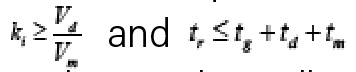

—in other words, equation 2 only applies when the analyte elutes during the period when the mobile phase arriving at the column inlet is actually changing with respect to time.

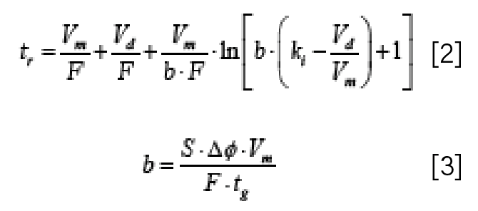

Looking at equations 2 and 3, we see that the dependence of the retention time and the GDV is complex, because Vd appears both outside and inside the log term. When the retention of an analyte is low in the mobile phase used as the starting point in the gradient (ϕi), and as ki approaches Vd/Vm, the influence of Vd on tr decreases. On the other hand, for compounds that are strongly retained and elute late in the gradient (that is, ki is large), then any change in Vd directly affects tr. For example, if Vd is 100 µL and the flow rate is 400 µL/min, then increasing Vd to 500 µL will increase the retention times of all compounds eluting late in the gradient by 1 min.
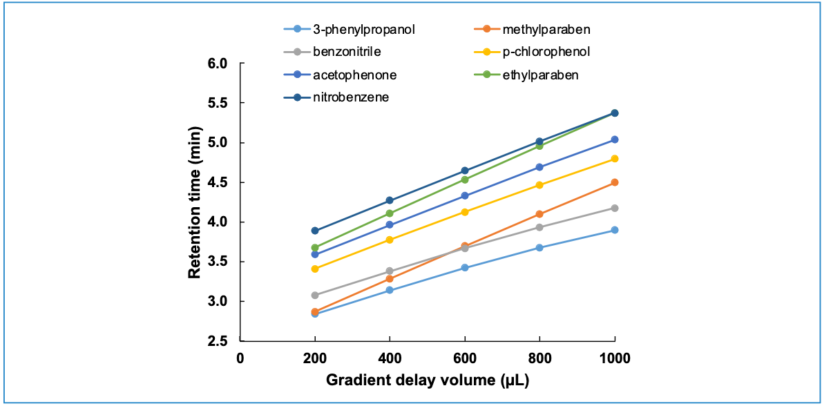
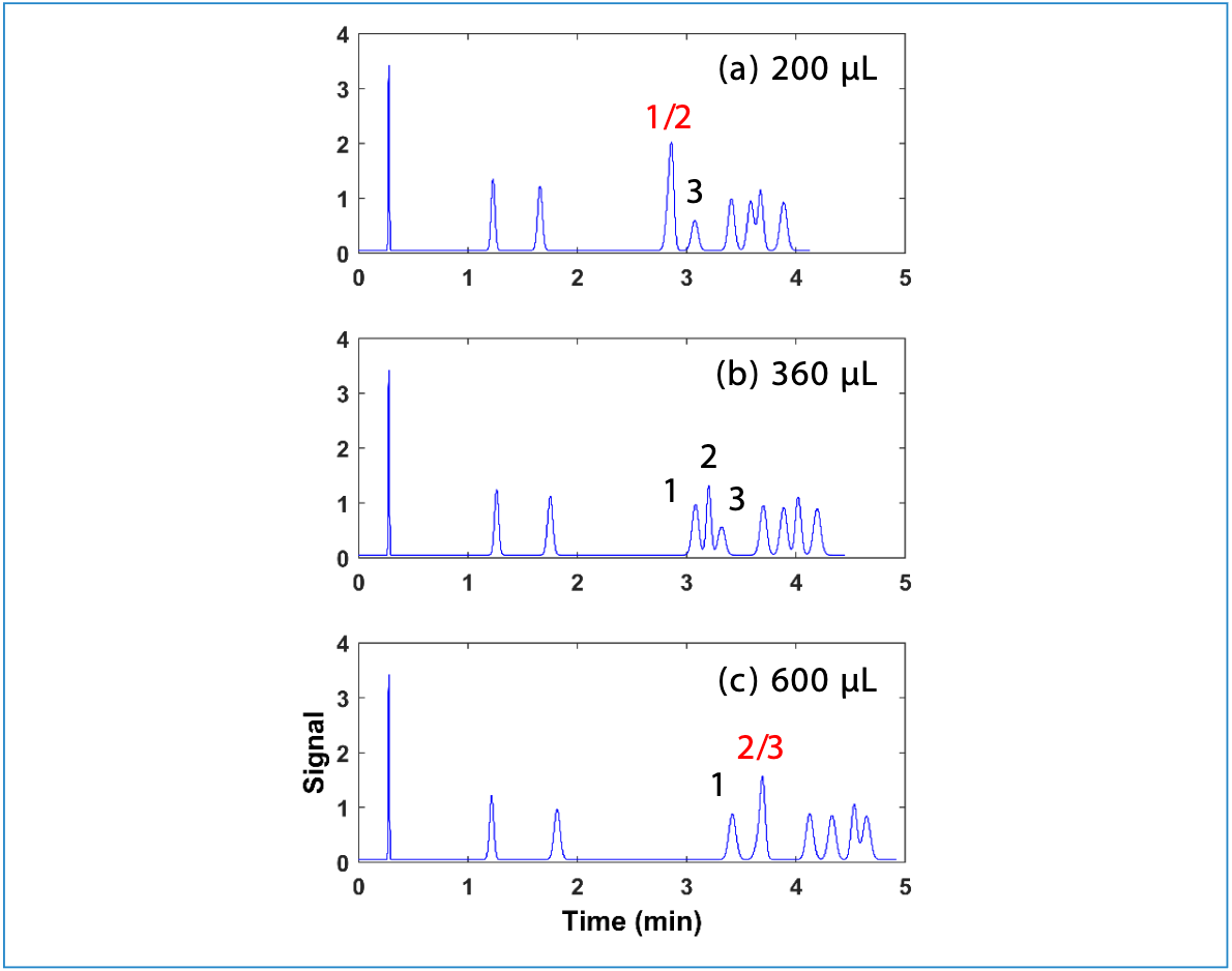
Now, the fact that the influence of Vd on retention time varies depending on where a compound elutes with respect to the gradient time, and the fact that S and ln(kw) influence retention time, means that there is the potential for Vd to influence not only retention time, but also selectivity. By using “selectivity” here, I mean that there is the potential for Vd to influence relative retention, and thus also resolution. The web-based HPLC simulator developed and maintained by my group (www.multidlc.org/hplcsim) is very useful for examining this type of phenomenon. The simulator is pre-loaded with retention parameters (which are calculated using LSS theory) that come from experimental measurements of retention time under reversed-phase conditions for about 40 small molecules, and we can simulate separations of these compounds while varying parameters such as flow rate, column dimensions, and GDV. Figure 3 shows the dependence of retention time on GDV for seven molecules. We see that in general retention increases with increasing GDV, as expected. However, the interesting thing is that some of the lines cross over each other, which is a result of the fact that different compounds have different sensitivities to changes in mobile phase composition, as measured by the S parameter in equation 1. Now, the practical consequence of this, of course, is that wherever two or more of the lines intersect, there will be coelution of the compounds corresponding to those lines. This is illustrated in Figure 4, which shows the simulated chromatograms that we would expect for systems with GDV values of 200, 360, or 600 µL. With GDV values of 200 or 600 µL, there is serious overlap of the peaks for 3-phenylpropanol and methylparaben or methylparaben and benzonitrile, and the three compounds in that region of the chromatogram are not resolved. At 360 µL, however, all three compounds are resolved with a minimum resolution of about 1.5. This illustration shows that the impact of the GDV on separation selectivity can be both a blessing and a curse. On one hand, this phenomenon can be leveraged during method development as a means of optimizing a separation. On the other hand, if we are simply trying to transfer an already-developed method from one instrument to another, this phenomenon could lead to complications during the transfer if the GDVs for the two systems are not the same.

. Chromatographic Parameters: Stationary phase, C18; Column dimensions, 50 mm x 2.1 mm i.d. (5 μm particle size); Flow rate, 0.4 mL/min; Temperature, 40 °C; Gradient elution from 10-50 %B from 0-5 min; A solvent, water; B solvent, acetonitrile. Red circles indicate coelution of 3-phenylpropanol and methylparaben (GDV = 200 μL) or methylparaben and benzonitrile (GDV = 600 μL); the green circle indicates that all three compounds are separated when the GDV = 360 μL.")
Figure 3: Dependence of retention time on gradient delay volume for several small molecules, obtained from simulations (www.multidlc.org/hplcsim). Chromatographic Parameters: Stationary phase, C18; Column dimensions, 50 mm x 2.1 mm i.d. (5 μm particle size); Flow rate, 0.4 mL/min; Temperature, 40 °C; Gradient elution from 10-50 %B from 0-5 min; A solvent, water; B solvent, acetonitrile. Red circles indicate coelution of 3-phenylpropanol and methylparaben (GDV = 200 μL) or methylparaben and benzonitrile (GDV = 600 μL); the green circle indicates that all three compounds are separated when the GDV = 360 μL.

 and (c) we see that there is coelution of compounds 1 and 2 or 2 and 3, but in (b) we see all three molecules separated with a GDV of 360 μL. Compounds 1, 2, and 3 are 3-phenylpropanol, methylparaben, and benzonitrile.")
Figure 4: Simulated chromatograms highlighting the influence of GDV on separation selectivity and resolution. Conditions are the same as those described in Figure 3. In panels (a) and (c) we see that there is coelution of compounds 1 and 2 or 2 and 3, but in (b) we see all three molecules separated with a GDV of 360 μL. Compounds 1, 2, and 3 are 3-phenylpropanol, methylparaben, and benzonitrile.
Some Practical and Non-Ideal Aspects of this Framework
How Can I Measure the Gradient Delay Volume for My LC System?
It is most common to determine the GDV for a LC system experimentally by spiking one mobile phase solvent with a tracer compound that can be detected easily and used as a proxy for the actual mobile phase composition. A commonly recommended setup for this is to use water as Solvent A and 0.1% acetone spiked into water as Solvent B. Then, after removing the LC column from the system, a gradient is run from mostly A to mostly B, and the absorbance of the column eluent is recorded at a wavelength where the tracer absorbs. This produces a result like the dashed trace in Figure 2 (see Figure 4 of reference 2 for an example of a real experimental result). When we make GDV determinations in my laboratory, we typically use 50:50 acetonitrile:water for Solvents A and B, and spike Solvent B with 10 µg/mL of uracil. We prefer to have some organic solvent in A and B to reduce adsorption of the tracer to system components, and we prefer uracil over acetone because uracil is quite stable in solution (unlike the volatile acetone), and these solutions can be used reliably over many months.
How Do I Know What the S and ln(kw) Values Are for the Compounds I’m Working With?
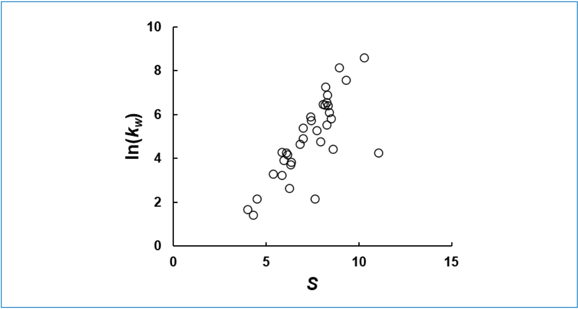
Figure 5 shows a plot of ln(kw) and S values calculated from experimental retention data for the same small molecules that are loaded into our HPLC simulator (www.multidlc.org/hplcsim). We see that they are correlated, and they give us a sense for the range of values typical of small molecules. However, I am not aware of any models that can predict the values for any combination of molecule, stationary phase, mobile phase, and operating conditions with enough accuracy to simulate separations of closely related compounds; at this point in time, the values must be determined by experiment, from retention data collected under either isocratic or gradient elution conditions. Readers interested in this process are referred to recent work that both discusses the process and its limitations (6).

 and S values for the 40 small molecules preloaded in our HPLC simulator.")
Figure 5: ln(kw) and S values for the 40 small molecules preloaded in our HPLC simulator.
Is ln(k) vs. ϕ really always linear?
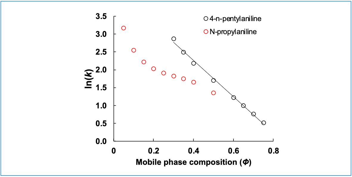
We observe very often that plots of ln(k) vs. ϕ are quite straight, at least over a range of ϕ relevant to practical separations, for small molecules and many biomolecules. An example of this is shown in Figure 6 for 4-n-pentylaniline. Sometimes, though, we observe that the relationship is nowhere near straight, as demonstrated in Figure 6 with the data for N-propylaniline, under exactly the same conditions. Building a highly accurate model in situations like this will require a non-linear model (for example, see the model of Neue and Kuss [7]); however, fitting even data like this to a linear model is good enough to support method development, provided that the user does not try to apply the model under conditions that are too far from the conditions used to collect the initial retention data (8).

.")
Figure 6: Experimental retention data for two small molecules illustrating varying degrees of linearity with respect to mobile phase composition. Conditions are the same as in Figure 3, except that mobile phase Solvent A is 25 mM ammonium formate, pH 3.2 (9).
Summary
In this installment of “LC Troubleshooting,” I’ve discussed the concept of gradient delay volume (GDV) and our understanding of its impact on retention and selectivity in reversed-phase separations, primarily from a theoretical point of view. The dependence of retention and selectivity on GDV can be leveraged to good effect during method development, but this same dependence can cause trouble during method transfer. In next month’s installment, I’ll discuss the practical implications of these aspects in more detail, including tips for troubleshooting problems related to the GDV, and best practices for avoiding GDV-related problems by transfer-proofing new methods during development.
References
(1) Snyder, L. R.; Dolan, J. W. High-Performance Gradient Elution: The Practical Application of the Linear-Solvent-Strength Model; John Wiley: Hoboken, NJ, 2007.
(2) Shoykhet, K.; Broeckhoven, K.; Dong, M. Modern HPLC Pumps: Perspectives,Principles, and Practices. LCGC N. Am. 2019, 37 (6), 374–384.
(3) Steiner, F.; Dong, M.; Paul, C. HPLC Autosamplers: Perspectives, Principles, and Practices. LCGC N. Am. 2019, 37 (8), 514–529.
(4) Seidl, C.; Bell, D. S.; Stoll, D. R. A Study of the Re-Equilibration of Hydrophilic Interaction Columns with a Focus on Viability for Use in Two-Dimensional Liquid Chromatography. J. Chromatogr. A 2019, 1604. DOI: 10.1016/j.chroma.2019.460484
(5) Schoenmakers, P. J.; Billiet, H. A. H.; Tussen, R.; De Galan, L. Gradient Selection in Reversed-Phase Liquid Chromatography. J. Chromatogr. A 1978, 149, 519–537. DOI: 10.1016/S0021-9673(00)81008-0
(6) Brau, T.; Pirok, B.; Rutan, S.; Stoll, D. Accuracy of Retention Model Parameters Obtained from Retention Data in Liquid Chromatography. J. Sep. Sci. 2022. DOI: 10.1002/jssc.202100911
(7) Neue, U. D.; Kuss, H.-J. Improved Reversed-Phase Gradient Retention Modeling. J. Chromatogr. A 2010, 1217 (24), 3794–3803. DOI: 10.1016/j.chroma.2010.04.023
(8) den Uijl, M. J.; Schoenmakers, P. J.; Schulte, G. K.; Stoll, D. R.; van Bommel, M. R.; Pirok, B. W. J. Measuring and Using Scanning-Gradient Data for Use in Method Optimization for Liquid Chromatography. J. Chromatogr. A 2021, 1636, 461780. DOI: 10.1016/j.chroma.2020.461780
(9) Kempen, T.; Dahlseid, T.; Lauer, T.; Florea, A.; Aase, I.; Cole-Dai, N.; Kaur, S.; Southworth, C.; Grube, K.; Bhandari, J.; Sylvester, M.; Schimek, R.; Pirok, B.; Rutan, S.; Stoll, D. Characterization of a High Throughput Approach for Large Scale Retention Measurement in Liquid Chromatography; preprint; Chemistry 2023. https://chemrxiv.org/engage/chemrxiv/article-details/63d17301ae221a16d13d4d2f (accessed 2023-02-10).
About the Author
Dwight R. Stoll is the editor of “LC Troubleshooting.” Stoll is a professor and the co-chair of chemistry at Gustavus Adolphus College in St. Peter, Minnesota. His primary research focus is on the development of 2D-LC for both targeted and untargeted analyses. He has authored or coauthored more than 75 peer-reviewed publications and four book chapters in separation science and more than 100 conference presentations. He is also a member of LCGC’s editorial advisory board. Direct correspondence to: LCGCedit@mmhgroup.com
 in the pharmaceutical industry | Image Credit: © Vladimir Polikarpov - stock.adobe.com")


 setup for separation and analytical chemistry. | Image Credit: © Artur Wnorowski - stock.adobe.com")


LC–MS/MS-Based System Used to Profile Ceramide Reactions to Diseases
April 26th 2024Scientists from the University of Córdoba in Córdoba, Spain recently used liquid chromatography–tandem mass spectrometry (LC–MS/MS) to comprehensively profile human ceramides to determine their reactions to diseases.

High-Throughput 4D TIMS Method Accelerates Lipidomics Analysis
April 25th 2024Ultrahigh-pressure liquid chromatography coupled to high-resolution mass spectrometry (UHPLC-HRMS) had been previously proposed for untargeted lipidomics analysis, but this updated approach was reported by the authors to reduce run time to 4 min.


Traditional Chinese Medicine’s Effects on Liver Cancer Measured Using New UHPLC–QTOF-MS System
April 22nd 2024Scientists from Anhui University of Chinese Medicine in Hefei, China recently investigated the mechanisms behind what makes huachansu tablets, a type of traditional Chinese medicine (TCM), effective against liver cancer.