
|Articles|January 14, 2022
- January 2022
- Volume 18
- Issue 1
- Pages: 18–23
Tips & Tricks: A Few Things Molar Mass Distributions Can (and Can’t) Tell
Author(s)Wolfgang Radke
Advertisement
Gel permeation chromatography/size-exclusion chromatography (GPC/SEC) is the standard technique to derive molar mass distributions of polymers and macromolecules. However, there are several ways to display molar mass distributions, depending on the information one needs to extract from it. This instalment of Tips & Tricks will explain the benefits of a molar mass distribution over molar mass averages and the differences between the different representations of molar mass distributions.
Macromolecular samples are disperse in molar mass. Thus, specifying a single molar mass to a macromolecular sample is insufficient to describe its characteristics. Certain required information can only be obtained from the molar mass distribution. For example, registration of chemicals according to the Regulation concerning the Registration, Evaluation, Authorisation, and Restriction of Chemicals (REACH) in the EU requires determination of the amount of material below specific molar masses (1). USP and EP monographs for dextrans require the weight average molar masses to be calculated for
the high and low molar mass fractions of the sample.
Gel permeation chromatography/size‑exclusion chromatography (GPC/SEC) is the most important chromatographic separation technique for macromolecules, allowing the determination of molar mass distributions. From the molar mass distributions the molar mass averages can be calculated. Often uncertainties in the interpretation of distributions exist because of their different representations. The information provided by molar mass distributions—in addition to molar mass averages—will be described in the following text.
Benefit of Molar Mass Distribution Compared to Molar Mass Averages
Macromolecular samples are often characterized using averages, such as weight-(Mw) and number-average (Mn) molar masses. The ratio of weight- to number-average molar mass, known as the dispersity index Đ = Mw/Mn, is typically used to describe the width of a molar mass distribution.
Molar mass averages are often applied to compare samples. Differing molar mass averages correspond to different samples. However, identical averages do not necessarily indicate the existence of identical or even similar samples. Furthermore, Đ only provides a very rough indication on the width but not on the shape of the molar mass distribution. As an example, it is not clear if there is a uniform distribution
with a single maximum or if there are several maxima due to a multimodal distribution.
In fact, for a given combination of number- and weight-average molar mass as well as the resulting dispersity, there exists an infinite number of possible molar mass distributions. This is shown in Figure 1, where three different molar mass distributions are displayed. All three distributions correspond to the same weight- and the same number-average molar masses of 50,000 g/mol and 15,000 g/mol, respectively, resulting in the same dispersity index of 3.3.
While the average molar masses are identical, the molar mass distributions are clearly not. This shows that the information content of a molar mass distribution is much higher than that of simple molar mass averages.
In summary, the molar mass distribution contains much more information than simple molar mass averages and allows:
- Distinction between mono- or multi‑modal distributions;
- Identification of inflection points or shoulders in the molar mass distributions, which might provide information on the polymerization process, for example;
- Determination of the amount of material below or above certain molar mass limits. Such information is often required for registration purposes and cannot be derived from average molar masses, but only from the distribution;
- Determination of mass fractions or even average molar masses within certain molar mass ranges, allowing much more precise material specifications for critical applications.
Differential and Cumulative (Integral) Molar Mass Distribution
Obviously, the molar mass distribution tells us something about “the relative portions of molecules with a specified molar mass or with molar masses within a specified range” (2). Whether the relative portions relate to a specific molar mass or to a molar mass range depends on whether the molar masses are assumed to be discrete or continuous. In the former case, the molar masses can take on only discrete specified values, while in the latter case they can take any intermediate value.
In GPC/SEC, continuous molar masses are usually assumed, though in reality this is not the case. However, the assumption of a continuum of molar masses is frequently applied in polymer science as it eases calculations.
The term molar mass distribution is not precisely defined at this point. The distribution can be based on the number fraction of molecules or on the mass portion of molecules with molar masses within a specified range.
In GPC/SEC, the distribution function typically refers to the mass portion of material. The molar mass range of a typical industrial polymer sample usually covers orders of magnitude. Therefore, in GPC/SEC a logarithmic molar mass axis is usually chosen. The above discussed “mass portion of molecules” within a specified range yields a so-called differential molar mass distribution and results in the often-found, nearly bell-shaped curves. It should be stressed that the molar mass distribution derived by GPC/SEC usually does not represent the number of molecules within specified molar mass ranges (frequency distribution) but the mass (weight) fraction of these, though they can be transferred into each other.
Frequently, besides the differential molar mass distribution, the cumulative or integral distribution is displayed. This typical sigmoidal-shaped curve represents the integral across the differential molar mass distribution from zero to the selected molar mass. Thus, the sigmoidal curve represents the area under the differential molar mass distribution curve. Consequently, the integral molar mass distribution I(M) describes the mass fraction of material with a molar mass less than M, within the sample (Figure 2).
Cumulative or integral distributions are used frequently to determine information required to decide on whether new products fall into the category “polymer of low concern” (PLC) or whether a product needs to be registered according to REACH (1).
To allow for better data comparison, the molar mass distributions can be plotted using different scaling on the ordinate. As mentioned above, the molar mass distribution w(logM) represents the mass portion of material of a given molar mass. The area of w(log M) is normalized to unity. In Figure 3(a), the different peak heights are a consequence of the different peak widths. As the distributions are normalized to unity, the different peak widths are compensated by the peak height.
Some people prefer a normalization such that the peak maximum corresponds to 100% (norm. w[logM]) (Figure 3[b]). As an example, this allows the easy determination at which molar mass the mass fractions have decayed to a certain percentage of the sample’s most prominent molar mass fraction.
In contrast, the relative molar mass distribution (rel. w[logM]) (Figure 3[c]) provides a non-normalized distribution. The total area under the curve varies with the amount of injected sample. Such a representation can be useful, for example if molar mass distributions are to be compared at different conversions. In that case rel. w(log M) allows visualization of the change in molar mass distribution and conversion within the same graph.
It should be noted that the peak shapes and molar mass averages are not affected by the selection of the ordinate. Furthermore, the peak maximum of the molar mass distribution does not represent the molar mass of the most abundant molecules in the sample. It represents the molar mass of the molecules contributing the highest weight fraction to the sample.
Molar Mass Distribution and Detector Signal
To derive the molar mass distribution of an unknown sample, the sample’s detector signal is recorded as a function of elution volume. Based on the calibration curve, the elution volume axis is converted into a logarithmic-scaled molar mass axis (logM). At the same time, a transformation is applied to convert the detector signal into a relative concentration as a function of logM, in this case the molar mass distribution (3).
There are various detectors that can be hooked up to a GPC/SEC instrument. Besides the fact that the detector must be able to detect the eluting polymer fraction—which often is not possible using a UV detector because of a lack of chromophores—one must consider how the detector signal responds to the eluting molecules.
Usually, one differentiates between concentration detectors and molar mass sensitive detectors. Molar mass sensitive detectors, such as light scattering detectors, are applied to determine the molar mass of each eluting fraction without the need for a GPC/SEC column calibration curve constructed using several molar mass reference standards (4). Their signals are not meant to be transferred into a molar mass distribution. Thus, the following section does not apply to them but only to UV, refractive index (RI), or evaporative light scattering (ELS) detectors, or any other concentration detector.
At first glimpse the term concentration detector seems to be clear, as the higher the eluting concentration, the higher the signal. However, a second look is needed.
Concentrations can be defined either in mass concentrations (units of mass per unit volume) or as molar concentrations (units of moles per unit volume). Again, at first it does not seem to matter if one elutes a given number or mass of molecules, as the eluting mass is given by the number of molecules multiplied by their molar mass. However, when performing a GPC/SEC analysis, if identical numbers of molecules (identical molar concentrations) are eluted at different elution volumes, they correspond to different molar masses. Consequently, the mass concentrations differ.
This situation is depicted in Figure 4 where three different poly(methyl methacrylate) (PMMA) molecules have a different number of repeating units. Each molecule carries an UV-active phenyl group at the chain end. The phenyl group gives rise to a strong UV absorption at 254 nm, where the repeating units do not absorb. Thus, the UV-signal at 254 nm will be proportional to the number of eluting molecules, namely to the molar concentration of eluting species. In contrast, the signal of an RI-detector is proportional to the number of eluting repeating units, ignoring the effect of the end group as a first approximation. Thus, the RI-detector’s response is proportional to the eluting mass concentration. Consequently, the term concentration detector is not as clear as it seems to be.
The question of detector response has a significant influence on the resulting detector signals. Figure 5 shows the chromatograms of a mixture of two PMMAs started using an UV-active initiator. Clearly, the shapes of the detector traces differ from each other. At higher molar masses (low elution volumes), the intensity of the UV-signal relative to the RI is lower when compared to higher elution volumes (lower molar masses). For the same UV‑intensity at low elution volume (high molar masses), the number of repeating units is higher than at higher elution volumes (lower molar masses). Therefore, the relative RI-signal is higher at low elution volumes. Since the signal traces of RI and UV differ, the molar masses calculated from the respective signals differ as well. The molar mass, however, is a sample property that is not expected to depend on the type of detector applied. Thus, if UV- and RI‑detector traces differ, a second thought should be given to identify which signal to use for molar mass calculation.
Commercial GPC/SEC software expects the signal of the detector to be proportional to the mass concentration. This means that the detector needs to recognize the number of repeating units rather than recognizing the number of molecules eluting at a particular elution volume. In other words, a single chain of a given chain length has to yield the same signal strength as two molecules of half of the chain length.
Thus, care must be taken if detector traces between UV- and RI-detectors differ. The often-applied approach of simply choosing the less noisy signal is not recommended. As UV-signals tend to be more specific than RI-signals, the universal RI-signal should be preferred.
Summary
- The information content of the molar mass distribution is much higher than that of the molar mass averages.
- There exists an infinite number of distributions with the same combination of number- and weight-average molar mass.
- A molar mass distribution provides the mass fraction of molecules within a specified molar mass range. It does not show the number portion of molecules—though it can be calculated from the molecular weight distribution (MWD).
- GPC/SEC programs assume signals proportional to the mass concentration of eluting species.
- If UV- and RI-detector traces differ from each other, the RI-signal should be evaluated to derive molar mass distributions.
References
- D. Held, The Column 13(8), 9–13 (2017).
- R.G. Jones et al., International Union of Pure and Applied Chemistry, Compendium of Polymer Terminology and Nomenclature (IUPAC Recommendations 2008) (https://iupac.org/projects/project-details/?project_nr=2002-048-1-400
- P. Kilz and D. Held, The Column 10(22), 26–30 (2014).
- D. Held, The Column 5(4), 28–32 (2009).
Wolfgang Radke studied polymer chemistry in Mainz (Germany) and Amherst (Massachusetts, USA) and is head of the PSS application development department. He is also responsible for instrument evaluation and for customized trainings.
E-mail: [email protected]
Website: www.pss-polymer.com
Articles in this issue
over 4 years ago
Rising Stars of Separation Science: Hedvika Raabováover 4 years ago
Thermo Fisher Finalizes PPD Acquisitionover 4 years ago
Gerstel Group Changes Ownershipover 4 years ago
Novasep Invests €6 Million into Chasse-sur-Rhône Siteover 4 years ago
Vol 18 No 1 The Column January 2022 North American PDFover 4 years ago
Vol 18 No 1 The Column January 2022 Europe & Asia PDFAdvertisement


Advertisement
Advertisement
Trending on LCGC International
1
The Silent Crisis: Can The Demise of Chromatography Teaching in Universities Be Reversed?
2
Multiplexed HILIC-HRMS Method Quantifies LPC and CAR Biomarkers for HCC
3
GC-MS Reveals Regional Flavor and Aroma Shifts in Oranges
4
Micro-LC-MS/MS Links 2-AG to Depression, Not Migraine
5