
|Articles|March 1, 2008
- LCGC North America-03-01-2008
- Volume 26
- Issue 3
Petroleomics — MS from the Ocean Floor
Author(s)Michael P. Balogh
Recent work suggests that the practical value of hyphenated techniques is limited by difficulties inherent in achieving definitive compositional answers in general MS. This article argues that it is not impossible in certain cases.
Advertisement
The abstract might seem to contradict recent columns where, for example, a look at the work of Tobias Kind and others (1,2) suggests that the practical value of hyphenated techniques is limited by difficulties inherent in achieving definitive compositional answers in general mass spectrometry (MS) practice. But given knowledgeable hands and the most advanced instrumentation, it is not impossible to do so in certain cases. Much of this discussion was presented at CoSMoS 2007.
Michael P. Balogh
Although we most often associate the suffix "-omics" with biologically important protein studies in living systems, the concept nonetheless applies to large and diverse groups of compounds in other important areas. Ryan Rodgers heads a petroleum research group in Professor Alan Marshall's group at the National High Magnetic Field laboratory at Florida State University. He offers rare insight into the need for extremes of accurate mass measurement, and its attendant data handling, to characterize hydrocarbons in petroleum production. The search for increasingly scarce petroleum reserves has impelled developers to adopt deep and ultradeep-water production techniques, producing oil in 5000–10,000 feet of water and thereafter drilling 5000–20,000 feet into the Earth's crust. Such projects entail a $1 billion, or more, decision regarding whether to produce an oil reservoir. The extreme circumstances prohibit sending a diver down to address production issues and limits the resolution of seismic instrumentation needed to discern what the reservoir looks like. Seismic data are still obtainable and important however the quality of the data is limited by both the depth of the water and depth of the ocean floor sitting on top of the reservoir. When the chemistry is not well understood, unfortunate and costly things can happen as oil is removed from a reservoir. For instance, Rodgers' group investigates the chemistry associated with asphaltene deposition in deep, undersea, petroleum-delivery lines. Asphaltene deposition is a sort of coronary artery disease for the petroleum industry. Asphaltenes aggregate on the inside of pipes as they bring oil to the surface producing backpressure, clogging valves and putting pressure of a different sort on oil production. Because it is impractical to send a diver down to remedy the problem, Rodgers' goal is to find a way for workers to anticipate the problem before it becomes catastrophic. Without sufficient knowledge of the chemistry in the reservoir before attempting to extract it to the surface the oil company risks the need to station a cleaning vessel on the surface, above its production facility, at a cost of between a half-million to one million dollars a day to clean the pipes.
So how does the industry get information on such complex mixtures? The National High Magnetic Field laboratory's high-field Fourier-transform ion cyclotron resonance (FT-ICR) building houses both 9.4-T and 14.5-T FT-ICR mass spectrometers. The instruments are fitted with various ionization sources — atmospheric-pressure photoionization (APPI), electrospray (ESI), field desorption, and low-voltage electron ionization — a variety made necessary by the analytical complexity and diversity of problems encountered in petroleum assays.
Designing The Experiment
The studies focus on small molecules and the complete analysis of complex mixtures. You need only a single drop of crude oil to perform the analyses. That drop, which weighs about 30 mg, is then diluted to about 0.1 mg/ mL, so it yields about 300 mL of stock solution. Thereafter you perform an array of MS techniques on the stock-solution sample. These techniques include positive-ion ESI, negative-ion ESI, field desorption or low-voltage electron ionization, and APPI, and they yield thousands upon thousands of identified entities while consuming less than 1% of the original drop of crude oil.
Consider the design of the ion cyclotron. It ensures that the higher the field, the higher the resolution; the more ions you can pack into the cell, the higher the dynamic range. When analyzing oil we are dealing with numerous, closely related hydrocarbons. Nevertheless, the analytical approach resembles that of many other characterizations of closely related analytes. Complex mixture studies often require extended dynamic range, as in the case of drug metabolite studies. MS provides a wealth of information as well as the characteristics of the ionization method used. For instance, positive ESI is limited to ionizing analytes more basic than the solvent in which they are contained. So when you are looking at bases, you use positive ESI. But the converse is true when you are looking at acids. In that case, you use negative ESI.
These are the primary information levels derived from high-resolution MS analysis:
- Accurate mass, from which elemental compositions can be assigned.
- The compound class. For example, the presence of hydrazine carbon identifies ethyl benzene as a component of the hydrocarbon class.
- The number of rings and double-bond equivalents (DBE), or the Z-number, indicates the type of compound. For example, one ring and three double-bonds indicates a DBE of 4.
- The carbon number is simply the number of carbons in the molecule and the ratio of hydrogen but it can suggest the amount of alkyl substitution in the molecule.
Characterizing Very High Resolution and Mass Accuracy
We often encounter the terms high resolution and high mass accuracy. What do they mean in the context of this discussion? Practitioners using quadrupole and ion-trap mass spectrometers that, if found wanting in resolution, often turn to time-of-flight (TOF) or hybrid (Q-TOF) instruments. The latter instruments range from low resolution to moderate resolution, as we observed in an earlier column on these topics (3). With the advent of today's high resolution of FT-ICR mass spectrometers, even magnetic sector instruments, traditionally known for their high resolution, are essentially downgraded to moderate-resolution instruments.
As for mass accuracy, consider this analysis: Two baseline-resolved peptides having a mass difference in elemental composition of S2H8 versus N4O were acquired using FT-ICR (Figure 1) with a calculated high-resolution of 3.3 million. The mass difference of 0.4 mDa is minuscule. (For reference, the mass of an electron is 0.5 mDa, so these two baseline-resolved peaks differ in mass by less than that of an electron). On high-field systems, routine resolving powers with such instruments are on the order of a half-million to one million. But as we observed in previous columns, resolution does not provide much analytically unless mass accuracy accompanies it. Mass accuracies measured to hundreds of parts per billion can measure the mass to the fifth decimal place, enabling assignment of elemental compositions. Rodgers uses programs similar to those we have examined in this column that can propose structures from accurate mass. To do so, you simply limit the search to expect C, H, N, O, and S in the molecule, and the programs produce a combination that gives the accurate mass within the experimental errors. According to Rodgers, at that level of measurement, unlike low resolution instruments that can simply limit the possibilities, you get only one answer most of the time.
Figure 1
Just the mass defect alone — the amount that the accurate mass differs from the nearest nominal mass — can yield information on the type of materials you are looking at. So on the basis of mass defect analysis, sugars, lipids, hydrocarbons, and amino acids can be seen to reside in different areas of the narrow space defined by the mass defect spectrum. Such specificity enables use of the Kendrick mass analysis, which was introduced in the 1960s (4).
Discerning extreme accurate mass is a valuable tool because every atom has a different mass defect and the linear combination of atoms for things occurring in nature seldom overlap. So for a given combination of C, H, N, O, and S, every mass is unique. If the mass is measured accurately enough, its elemental composition is ascertainable. The exact mass (more appropriately, the calculated exact mass) is obtained by summing the masses of the individual isotopes of the molecule. For example, the exact mass of water containing two hydrogen (1H) and one oxygen (16O) is 1.0078 + 1.0078 + 15.9994 = 18.0106. Hydrogen has a positive mass defect, so hydrocarbons, as mass increases, "walk out" from the nominal mass (Figure 2). Sulfur, with a negative mass defect (as evident with benzothiophene and dibenzothiophene compounds) "walks" the other way relative to hydrocarbon compounds.
Figure 2
Looking at the nominal mass with all the possible combinations of C, H, N, O, and S, and placing the candidates in 1-mDa bins produces an extraordinary number of possibilities. When you zoom in on the spectral axis, the mass spectrum reveals "gaps," and the number of possibilities for elemental compositions in every millidalton bin is, on average, four or greater. Even for 0.5-mDa bins, the number of possibilities is still too many to be useful. But at 0.1-mDa bins, most of the mass space is empty where having "spaces" in the spectral range containing no masses enables a unique elemental-composition assignment for things that do not have only C, H, N, O, and S (Figures 3 and 4). At 0.1-mDa mass accuracy and mass 500, we "typically" see one possibility. Rodgers says, "I could tell you from experience if you have two or even three possibilities for elemental composition, that using simple, rational bond rules and what's allowed in nature can lead you to a unique solution to the problem. You need plus or minus 100 ppb, if you have every single possibility of C, H, N, O, and S. And we know that that's not true in nature. Nature is very complex. But she's not that mean."
Figure 3
What is the advantage of increasing an already high magnetic field when you go from a 9.4-T instrument to a 14.5-T one? The answer to a question of analytical interest sheds some light: how complex are the complex mixtures that you are going to analyze?
Figure 4
A photoionization experiment done in negative ion detection mode on South American crude oil shows nearly 12,500 assigned masses in the mass spectrum (Figure 5). These masses are resolved and identified at the level of elemental composition assignment. Plotting the mass error relative to the measured mass produces a pseudo-Gaussian profile centered, approximately, on zero; the width of this peak is ±200 ppb. As Rodgers observes, "Nature is not so cruel to allow every combination of C, H, N, O, and S. But she is not too nice either, giving you something like a factor of two in the difference of what you need and what you can do." That said, it is nevertheless true that such a close level of observation can fetch a unique elemental-composition assignment for anything.
Figure 5
The same experiment using ESI produces spectra for 11,000 bases using positive-ion acquisition and another 6000 acids using negative-ion acquisition modes. So from a single sample, 30,000 chemical entities are identifiable — from acids to bases to aromatics. For the most part, the approach is orthogonal because, as Rodgers says, "In ESI negative mode, you are looking at acids. You are not going to see them in positive ESI (which are the bases). In APPI mode, you're looking at mostly hydrocarbons and nonpolar sulfur, which you are not going to see in either ESI mode. So you really get a ton of information and very little compositional overlap."
Compared with a 9.4-T instrument, a 14.5-T instrument shows a 100-fold decrease in ion accumulation time, a twofold increase in detection time, a 30-fold better external calibration, and a 20-fold decrease in analysis time. A recent example showed 28,400 spectral peaks resolved and identified at three sigma from the baseline noise resolving power of approximately a half-million from a single peak. According to Rodgers, a single experiment is now approaching the point where it equals the work we previously achieved in three experiments using different ionization modes. In numbers, that implies the capacity to identify 35,000 things in a single mass spectrum.
Deducing Information from Data
Echoing a recent column's statement on Tobias Kind's work (2), how do we manage data and display it? It would indeed be wondrous to resolve all these peaks. But we find ourselves at a technological impasse when we try to do so. Assuming a throughput rate of 25 to 30 samples/day and 10,000 peaks/scan (a conservative estimate), we cannot even conceive of the enormity a task that assigns the correct elemental composition to a quarter million peaks per day. So we need workarounds. Rodgers uses Van Krevelen diagrams to arrange the raw elemental composition data and display compositional trends of interest. Plotting the H:C ratio versus the O:C ratio, the Van Krevelen diagram spreads out the various homologous series. He then color codes these series according to their relative abundance (Figure 6) to visualize differences: for example: O, O2, O3, O4. Thus, he converts a complex mixture into an image. If, say, he wants to look at how things vary in a specific class, he can use the N, NO, NO2, NO3 series.
Figure 6
Rodgers also uses two-dimensional and three-dimensional Kendrick diagrams. Using the IUPAC mass, normalized to a CH2 unit as exactly 14 (so that every time a CH2 adds, no mass defect is accumulated) makes the data linear. He says you can convert raw data to an image by considering the Kendrick mass defect versus nominal mass and then color coding the peaks and contour plotting them. But he does not follow that route because, as he puts it, "it is hard on your PC." So he simply makes them two-dimensional, looking at them from above. He then uses color for the third dimension (Figure 7), a DBE essentially defines how aromatic an entity is, and a carbon number reports the amount of carbon in each elemental composition. These are extremely useful techniques, Rodgers says. When viewed in terms of low temperature versus high, you observe two different responses. In the middle of those temperatures, two stable, core structures, which differ by approximately 4 DBE — the difference of a benzene molecule — appear. In essence, says Rogers, you are looking at the exponential growth and evolution of related polycyclic aromatic hydrocarbon (PAH) compounds produced in the distillation process in the presence of thousands of peaks. A note of interest. As this column was in process I found in October 2007, Sierra Analytics, Inc. announced an exclusive licensing agreement with Dr. Rodgers and Florida State University to bring petroleomics software to the commercial marketplace. Dr. David Stranz, Sierra's president, said "We are excited to be collaborating with Dr. Rodgers and the NHMFL on this new software. Until now, no software capable of analyzing and visualizing petroleomics data has been commercially available." Sierra expects to release the first version of the software in June 2008.
Figure 7
Detecting "Coronary Artery Disease" in Pipelines
Quick looks at just the classes indicates the presence of deposited asphaltenes, many species of which evidence multiple hetero atoms and tend to be more polar (not completely unexpected). How do they differ in DBE or carbon number? Looking at every nominal mass to answer that question would take a very long time. As hydrogen is added, a positive mass defect results, and species move to the right. Conversely movement to the left implies less hydrogen. More aromaticity implies multiple hetero atoms per assigned peak.
Identifying the culprit
The crude oil in a reservoir is at high temperature and high pressure; the pressure must be reduced to get oil out. But reducing pressure can create a problem. When pressure starts to bleed, asphaltenes can flocculate, drop out of solution, become sticky, and start plating on pipe walls. Unlike laboratory control samples, it becomes immediately obvious by examining the various classes of asphaltenes that naturally occurring asphaltenes are entirely different samples. The pressure-drop asphaltenes being removed from the earth are highly enriched in oxygen functionalities whereas the dead-oil asphaltenes are mostly nitrogen based. The pressure-drop asphaltenes are relatively low in Kendrick mass defect, so they are not especially aromatic. If you look at the laboratory-prepared, solvent-drop asphaltenes, you can see they shift up and are far more aromatic than the pressure-drop species. The compositional difference in the pressure drop asphaltenes identifies the species responsible for the formation of the initial "flocs." Such information is invaluable in the design of chemicals that could be used to prevent formation of the deposits.
According to Rodgers, low-resolution instruments still have their place, even in petroleum research. "I use them routinely for MSn. But you really, really must be careful when you are looking at complex mixtures. Aggregation and other concentration-dependent things can cause enormous deception. In one case, looking at a low-resolution mass spectrum, it appeared the acids ranged from 200 to 2000 Da. Nevertheless, the FT-ICR indicated they were about 350 to 800 Da. In this case, acquiring a high molecular weight sample and just barely fragmenting — and we have done 15 different standards to assure ourselves that covalent bonds do not break when you do this — disrupts only noncovalent interactions. Consequently, the molecular weight is seen diminishing. So you can re-isolate and do the fragmentation experiment in succession (MS4), and get exactly what you would, essentially, with a high resolution instrument. So you really need to be careful in mass spectrometry when you're looking at complex mixtures because they can do things that you don't expect."
A questioner asked Rodgers at CoSMoS 2007 whether he ever considers using chromatography. For biological applications, where the dynamic range can be 106, or higher, between the most abundant and least abundant species in solution, chromatography is indispensable. But petroleum samples are free of the problems associated with concentration and dynamic range. So "diluting and shooting" is far easier than performing chromatography. "One of the huge advantages of high-field work is that high-resolution works on a chromatographic time scale: you simply do not need to (acquire data for as long as one does in a chromatographic run) to realize the same benefit."
Why is there so little overlap in the positive ESI, negative ESI and APPI? Rodgers responds that nature has "beaten up" these molecules for millions upon millions upon millions of years. So they are at the global minimum in their structure, beat into pyrodenic, pyrolic, carboxylic acid, phenol, standard PAH, PASH, PANH type forms. When you look for overlap, even with standards between those entities, you are disappointed. And when you look at positive ESI, you are looking at the pyrodenic forms. When you look at negative ESI you are looking at the pyrolic nitrogen and the carboxylic acids. When you switch to APPI you are looking mostly at the hydrocarbons and the nonpolar sulfur.
Now 30,000 peaks do not appear in the APPI or positive ESI mass spectrum without any overlap. It definitely occurs in the nitrogen series, then pyrodenic and pyrolic. But the overlaps do tend to be less abundant. So the dynamic range actually works in your favor because the things that you want to see are present in higher concentration. So when you tune the ionization for aromaticity, the nitrogen compounds fall out because they are not as abundant as the PAHs and PASHs."
Michael P. Balogh
"MS — The Practical Art" Editor Michael P. Balogh is principal scientist, MS technology development, at Waters Corp. (Milford, Massachusetts); President and co-founder of the Society for Small Molecule Science which organizes the annual CoSMoS conference; and a member of LCGC's editorial advisory board.
References
(1) M.P. Balogh, LCGC24(8),762–769 (2006).
(2) T. Kind and O. Fiehn, LCGC26(2), 176–187 (2008).
(3) M.P. Balogh, LCGC22(2), (2004).
(4) E. Kendrick, Anal. Chem. 1963, 35, 2146–2154.
Articles in this issue
over 18 years ago
New Chromatography Columns and Accessories at Pittcon 2008: Part Iover 18 years ago
Peaks of Interest- Breath Test Diagnosis for Diseasesover 18 years ago
Peaks of Interest- MIT Develops Tiny Gas Sensorover 18 years ago
Amino Acid Analyzersover 18 years ago
Recent Developments in High-Abundance Protein Removal Techniquesover 18 years ago
Atmospheric Pressure Photoionization — The Second Source for LC-MS?over 18 years ago
Method Transfer ProblemsAdvertisement
Related Content
Advertisement


Advertisement
Advertisement