Treat It Like a Circuit, Part II: Applications and Troubleshooting

In this installment, we apply the concepts developed in last month’s installment by demonstrating how they can be used to help troubleshoot problems in LC involving pressure and flow.
The analogy that electrons flowing in wires is like water flowing through a tube can be remarkably effective for teaching and learning about fluid flow in LC systems. In this installment, we apply the concepts developed in last month’s installment by demonstrating how they can be used to help troubleshoot problems in LC involving pressure and flow. We also introduce several free tools that can be used to calculate pressure drops in different elements of LC systems, including connecting capillaries and packed columns. Knowing what pressure drops to expect for system components under different chromatographic conditions is very valuable in many troubleshooting situations.
In last month’s installment of “LC Troubleshooting,” we discussed the conceptual similarities between the flow of current in electrical systems and the flow of fluids in LC systems. We also discussed several basic principles and laws used to explain the behaviors of electrical systems, with the promise that similar relationships can be used to rationalize observations related to flow and pressure in LC systems, particularly as it relates to troubleshooting problems related to flow and pressure. In this installment, we continue this discussion, using several examples to illustrate how the principles discussed last month can be used to systematically explain the behaviors of flow and pressure in situations of great practical value. These include diagnosing situations where the measured pressure in a LC system appears to be too high or too low and setting up a passive flow split at different points in the flow path from pump to detector. As part of these discussions, we will also demonstrate the utility of freely available calculators that have been developed for the purpose of calculating pressure drops in LC systems.
Review of Concepts From Part I
Here, we reiterate the essential elements of the principles and relationships discussed in Part I for convenience. However, we strongly encourage readers who are unfamiliar with them and have not read Part I to pause and read through Part I before attempting to work through the examples in this installment. A major point of this two-part series is to provide the framework and principles needed to approach flow and pressure problems systematically; this is not possible without a firm understanding of the fundamental principles discussed in Part I.
In electrical systems, current flows through resistive elements (that is, wires and other electrical components that have some intrinsic resistance to the flow of electrons through them) as a result of the voltage drop across those elements. The analogous concept in fluidic systems is that fluid flows through resistive elements (that is, tubes and other fluidic components that have some intrinsic resistance to the flow of fluid through them) as a result of pressure drops across those elements. Two foundational tools used in the analysis of electrical systems are Kirchhoff’s Voltage and Current Laws. The Voltage Law asserts that the sum of the voltage rises and voltage drops encountered in a loop of the circuit must be zero. The Current Law asserts that the sum of all currents flowing into a junction point in a circuit must be equal to the sum of all currents flowing out of that same junction; this is an expression of the idea that charge must be conserved in any closed system. We can apply the concepts underlying these laws to fluidic systems as well. In that case, we would say that the sum of all the pressure rises and all the pressure drops encountered in a loop in the system must be zero. Subsequently, we would say that the sum of all the flow rates of streams entering a junction point in the system must be exactly equal to the flow rates of all the streams exiting that same point; there is a conservation concept at work here as well, and that is the conservation of mass. In the next sections, we explicitly show how these ideas can be employed systematically to address practical aspects of LC systems.
Using the Concepts to Troubleshoot Common Problems Related to Flow and Pressure
Pressure That Appears to Be Too High
There are many potential causes of pressure that appears to be too high. The list of these causes, and the steps to investigate them, is well established (1). However, the major problem in troubleshooting practice is that the number of places where there can be a pressure problem is also large, and identifying which is the important one, or whether there are actually multiple problems, can take some time. This is mainly because most LC systems only have one pressure sensor near the pump, which is almost always upstream from the sampler.
Figure 1a shows a schematic of a typical flow path for an LC system. The expected total pressure drop for this flow path, including the column, is 252 bar when the flow rate is 2.0 mL/min (see the next section for discussions about where this expectation comes from and free tools for calculating the pressure drops). In this case, for simplicity of demonstration, the pressure drop is calculated for a mobile phase with a viscosity of 1 cP, which is close to the viscosity of water at room temperature. Now, suppose that we encounter a situation where the pressure measured at the pump is 375 bar–123 bar higher than normal, as shown in Figure 1b. For example, this deviation is far more than we would expect to result from small changes in laboratory temperature. Again, the trouble at this point is that we don’t know which of the resistive elements in the flow path is causing the higher-than-expected pressure because we only have one pressure measurement—the total drop across the entire flow path. So, we need to break down the problem, and the easiest way to do this is to remove one or more elements of the flow path and record the new pressure. Figure 1c shows that when we remove all the elements downstream from the inline filter (see reference [2] to learn more about inline filters), the pressure drops by 213 bar to 162 bar, but this alone does not tell us much about specific elements. However, if we then remove only the inline filter, we obtain a critically important piece of information. Figure 1d shows that the pressure drops by 48 bar when the filter is removed; now, we can apply the fluidic equivalent of Kirchhoff’s Voltage Law, which we discussed in last month’s installment. That relationship tells us that pressure drops ΔP1 and ΔP2 add to give the total pressure drop ΔPT, and thus ΔP2 = ΔPT – ΔP1 = 48 bar. Now, from experience, we know that the pressure drop across this inline filter is approximately 5 bar when it is new and not at all occluded. So, the fact that the observed pressure drop across the filter is 48 bar means that the filter is partially occluded and should be replaced. We could try backflushing the filter to remove debris and decrease the pressure drop; however, in our experience, this is usually only partially successful, and usually a very short-term fix. It is far more effective to simply replace the filter.

 Complete illustration of all the resistive elements in the flow path. (b) Pressure measured at the pump indicates a pressure that is 123 bar higher than normal. (c) The total pressure drop decreases by 213 bar when all elements after the inline filter are removed from the flow path. (d) Removing the inline filter further decreases the pressure drop by 48 bar, which is 43 bar higher than the pressure drop expected for the filter itself. (e) Removing the capillary that normally connects the sampler to the filter further reduces the pressure drop by 80 bar, which is 60 bar higher than the expected pressure drop for the capillary itself.")
FIGURE 1: Flow diagrams for the flow path in a simple LC system at several stages of the process of troubleshooting an apparent high pressure problem. (a) Complete illustration of all the resistive elements in the flow path. (b) Pressure measured at the pump indicates a pressure that is 123 bar higher than normal. (c) The total pressure drop decreases by 213 bar when all elements after the inline filter are removed from the flow path. (d) Removing the inline filter further decreases the pressure drop by 48 bar, which is 43 bar higher than the pressure drop expected for the filter itself. (e) Removing the capillary that normally connects the sampler to the filter further reduces the pressure drop by 80 bar, which is 60 bar higher than the expected pressure drop for the capillary itself.
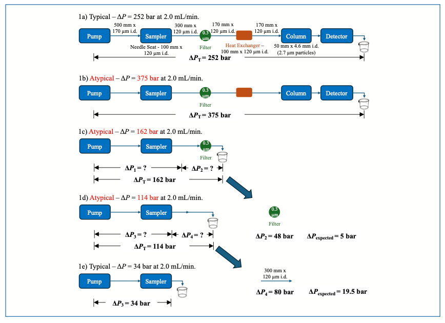
At this point, the total pressure drop from the pump to the outlet of the capillary connecting the sampler to the inline filter is 114 bar (Figure 1d). This still seems like too much, which we might know either from experience at looking at the elements involved, reviewing prior measurements made using this system, or from calculations of the pressure drops expected for individual elements (see the next section for discussion of calculated pressure drops). In any case, we can continue checking individual elements by removing them from the system one at a time and recording the new pressure. In Figure 1e, we see that when the 300 mm x 120 µm i.d. capillary is removed from the outlet of the sampler, the pressure drops by another 80 bar. We know from our favorite calculator tool that the expected pressure drop is just 19.5 bar–60 bar lower than what we have observed. Again, we could try backflushing the capillary to recover it, but this is likely to be only partially successful, and it is usually better to simply replace the capillary.
If we are interested in a comprehensive assessment of all the elements of the flow path, we would need to record the pressure drops observed after removing each element one at a time, starting with the detector and moving all the way back to the pump. In practice, we observe that most problems with high pressure because of occlusion of elements in the flow path occur between the sampler and the column inlet. Problems can occur between the pump and sampler, and downstream from the column, but these are less common because the column itself acts like a filter, and the mobile phase leaving it generally carries less debris than the mobile phase entering it.
Pressure That Appears to Be Too Low
Pressures that appear to be too low almost always indicate a leak somewhere downstream from the pressure sensor in the pump. One way of thinking about this is that the leak is an unintended flow split (see the section below and Figure 4 regarding passive flow splitting). If the flow rate through the split path exiting the split junction is not zero, then the flow rate through the main path to the detector must be less than the total flow entering the split junction. The lower flow in the main path will lead to a lower-than-expected pressure drop across that part of the flow path and a lower overall pressure drop measured at the pump.
Free Calculators That Support the Use of the Concepts
Capillary Flow and Mass Rate Calculator (Pacific Northwest National Laboratory)
The functionality for calculating pressure drops across both open tubes (that is, connecting capillaries used in LC) and packed columns is available in the Molecular Weight Calculator package (developed using Visual Basic, and downloadable for location execution) developed by researchers at the Pacific Northwest National Laboratory (PNNL–https://pnnl-comp-mass-spec.github.io/Molecular-Weight-Calculator-VB6/). The open tubular column feature is most accurate and can provide the estimated pressure drop for a given capillary inner diameter and length, in addition to the flow rate through the tube. Keep in mind that the actual diameters of manufactured tubes can be slightly different from the advertised diameter. This variation becomes more important as the diameter becomes very small (for example, below 75 µm i.d.). The packed column feature gives estimates for pressure drop at a given flow rate, column dimensions, particle diameter, and interstitial porosity (that is, the fraction of the column volume that is the space between the particles) using the Kozeny-Carman and Darcy equations (3). The column dead time and volume calculations are designed for columns packed with nonporous particles, which is atypical for most commercial columns, and thus, not as accurate for columns packed with porous particles. The most important upside of this calculator is that estimates for both connecting capillaries (that is, “open tubes”) and packed columns can be made using this one easy-to-use tool.
Web-Based Dispersion and Pressure Drop Calculator (Stoll Laboratory)
The web-based tool developed by the Stoll Group mainly for the purpose of dispersion calculations (https://www.multidlc.org/dispersion_calculator/; [4–7]) also provides pressure drop calculations for open tubes. Figures 2 and 3 show screenshots of the inputs available to the user, and the pressure drops for each element of the system provided as outputs. The major upside of this tool is that pressure drops can be calculated for multiple elements at one time, and the output provides a kind of system-level view for both dispersion and pressure drop. This tool was used to calculate all the pressure drops across connecting capillaries shown in Figure 1 and discussed in the previous section.

.")
FIGURE 2: Screenshot of the input array available to users in the “Dispersion Calculator” (https://www.multidlc.org/dispersion_calculator/).
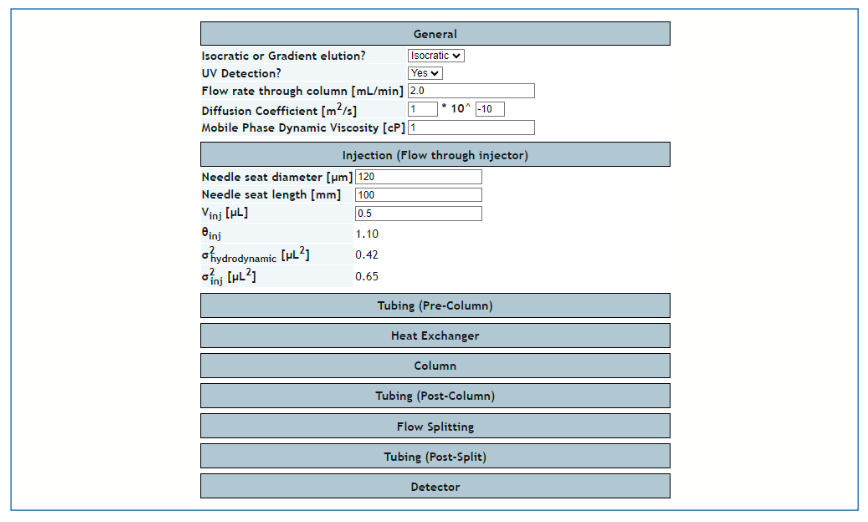


FIGURE 3: Screenshot of the pressure drop outputs provided by the Dispersion Calculator.

Web-Based HPLC Simulator (Stoll Laboratory)
The web-based HPLC simulator maintained by the Stoll Group (https://www.multidlc.org/hplcsim/; see [8] for detail about how it works) also provides a means to calculate pressure drops across packed columns. An upside of this tool relative to the others already mentioned here is that the intraparticle porosity can also be specified, which affects the column dead volume estimate but not the pressure drop. The simulator calculates the mobile phase viscosity, which is needed for the pressure drop calculation, based on the temperature and mobile phase composition (that is, the organic solvent-to-water ratio) inputs, which is a convenient feature.
Application of the Concepts to Passive Flow Splitting
Aside from troubleshooting problems related to higher-than-expected pressures, one of the other places where the concepts discussed in last month’s installment are often at play in the practice of LC is instances where passive flow splitting is used. By “passive,” we mean that the split ratio is not actively controlled by a pump or some other mechanical device. Rather, the split ratio is simply a result of the nature of flow through two open tubes. Passive flow splitting is most commonly used when an LC method running a relatively high flow rate (for example, much higher than 500 µL/min) is coupled with mass spectrometric (MS) detection where a lower (typically lower, but sometimes much lower, than 500 µL/min) flow rate is desirable for the detector.
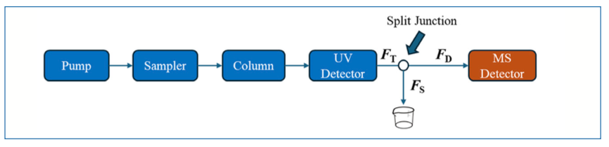
A simple schematic of an LC–MS system involving passive flow split prior to the MS detector is shown in Figure 4. Here, we refer to the total flow rate of mobile phase exiting the LC system as FT, and the flow rates through the connection to the MS, and to waste, as FD and FS, respectively. Now, usually the outlets of both the capillary carrying the split flow FS and the outlet of the capillary connecting to the MS are very close to atmospheric pressure, such that the pressure drops from the split junction to these points must be equal, as expressed in equation 1:


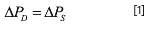


FIGURE 4: Simple schematic of a flow path commonly used for LC–MS, highlighting important details related to passively splitting the flow prior to the MS detector.
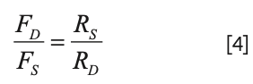
In each case, the pressure drop is the product of the flow rate and the flow resistance (that is, the fluidic equivalent of Ohm’s Law, discussed in Part I of this series):


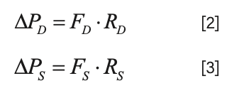
However, since the pressure drops are equal, we can relate the ratio of the flow rates to the ratio of the resistances:


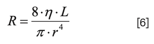
Now, the details of the resistance of each branch are given by Poiseulle’s Law (see Part I for a more detailed discussion):


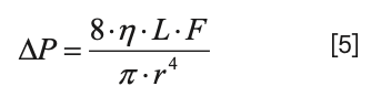
If we pull out the resistance piece, we have:


Substituting this back into equation 4, we find that only the length and radius (and therefore, diameter) of the capillaries connecting to the split point determine the ratio of the flow rates through the two branches (assuming that the viscosity of the fluid in the two branches is the same, which is correct in the vast majority of practically relevant uses of flow splitting at the inlet to a detector):


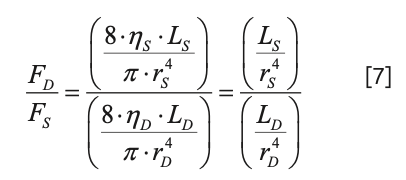
If the same tubing diameter is used for both capillaries, then equation 7 reduces even further to:


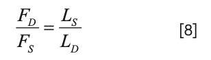
For example, if we wanted to split a 2 mL/min flow rate coming from the LC such that 500 µL/min goes to the MS and 1.5 mL/min goes to waste, we would simply choose lengths of the same diameter capillary to connect to the MS and to waste such that the ratio is 3:1, as shown in equation 8 (for example, 300 mm and 100 mm).
While this turns out to be beautifully simple, we should be careful. In some prior work (9), we showed that use of long tubes to connect the split junction to the MS can lead to really devastating peak broadening. Thus, in practice, we find a combination of capillaries that varies both in length and diameter while still satisfying the ratio in equation 7, such that we can make the length and volume of the capillary connecting the split junction to the MS as low as practically possible.
Summary
In this installment, we have reviewed the idea that concepts from electronics can be used to help understand the relationship between flow and pressure in LC systems, and then applied those concepts to two commonly encountered situations impacting pressure and flow. When troubleshooting higher-than-expected pressures, the idea that the pressure drops across each element of the flow path add to produce the total pressure drop measured at the pump is essential to a systematic approach to understanding which element of the flow path is producing the problem. We also briefly discussed several free calculation tools designed to calculate pressure drop across both open tubes (that is, connecting capillaries) and packed columns. These tools are very helpful in that they can help us understand what pressure drops to expect for a given set of conditions, and these expectations can help us discern whether or not there is a pressure problem at all. Finally, we’ve discussed a systematic approach to setting up a passive flow split that is often used to connect an LC system running at a flow rate that is too high for a MS detector. We hope that these detailed discussions will enable readers to apply the concepts relating flow and pressure to other situations they encounter in their use of LC.
Acknowledgements
The Pacific Northwest National Laboratory is acknowledged for developing and hosting the Molecular Weight Calculator and Capillary Flow and Mass Rate Calculator (https://pnnl-comp-mass-spec.github.io/Molecular-Weight-Calculator-VB6/).
References
(1) Stoll, D. R. Essentials of LC Troubleshooting, Part I: Pressure Problems. LCGC North Am.2021, 39 (12), 572–574.
(2) Stoll, D. R. Filters and Filtration in Liquid Chromatography– What to Do. LCGC North Am.2017, 35 (2), 98–103.
(3) Carr, P. W.; Stoll, D. R. Chapter 2: Speed and Performance in Liquid Chromatography. In Multi-Dimensional Liquid Chromatography: Principles, Practice, and applications; CRC Press: Boca Raton, FL, 2022.
(4) Stoll, D.; Broeckhoven, K. Where Has My Efficiency Gone? Impacts of Extra-Column Peak Broadening on Performance, Part I–Basic Concepts. LCGC North Am.2021, 39 (4), 159–166.
(5) Stoll, D.; Broeckhoven, K. Where Has My Efficiency Gone? Impacts of Extra-Column Peak Broadening on Performance, Part II–Sample Injection. LCGC North Am.2021, 39 (5), 208–213.
(6) Stoll, D. R.; Broeckhoven, K. Where Has My Efficiency Gone? Impacts of Extracolumn Peak Broadening on Performance, Part III: Tubing and Detectors. LCGC North Am.2021, 39 (6), 252–257.
(7) Stoll, D. R.; Lauer, T. J.; Broeckhoven, K. Where Has My Efficiency Gone? Impacts of Extracolumn Peak Broadening on Performance, Part IV: Gradient Elution, Flow Splitting, and a Holistic View. LCGC North Am.2021, 39 (7), 308–314.
(8) Abate-Pella, D.; Stoll, D.; Carr, P.; Boswell, P. An Open-Source Simulator for Exploring HPLC Theory. LCGC North Am.2015, 33 (3), 200–207.
(9) Gunnarson, C.; Lauer, T.; Willenbring, H.; Larson, E.; Dittmann, M.; Broeckhoven, K.; Stoll, D. R. Implications of Dispersion in Connecting Capillaries for Separation Systems Involving Post-Column Flow Splitting. J. Chromatogr. A 2021, 461893. DOI: 10.1016/j.chroma.2021.461893
ABOUT THE AUTHORS


Dwight R. Stoll is the editor of “LC Troubleshooting.” Stoll is a professor and the co-chair of chemistry at Gustavus Adolphus College in St. Peter, Minnesota. His primary research focus is on the development of 2D–LC for both targeted and untargeted analyses. He has authored or coauthored more than 99 peer-reviewed publications and four book chapters in separation science and more than 150 conference presentations. He is also a member of LCGC’s editorial advisory board.
chroncich@mjhlifesciences.com


James P. Grinias is a professor in the department of Chemistry & Biochemistry at Rowan University in Glassboro, New Jersey.