
|Articles|March 1, 2022
- March 2022
- Volume 40
- Issue 3
- Pages: 136–139
Enter the Matrix: Improving the Interpretation of Separations Data Using Chemometrics in Analytical Investigations

Advertisement
This article describes a compendium of chemometrics applications in separation science to demonstrate the importance and synergy of data handling. We review the main points that must be raised when using multivariate techniques and list references for further reading. With examples in food science, the case studies comprise of applications of pattern recognition (principal component analysis, PCA), regression (partial least squares, PLS), and classification methods (soft independent modelling of class analogies, SIMCA).
Analysts are often challenged by the multidisciplinary aspects of qualitative investigations, which require a broad set of skills. In this context, it is important to recognize the synergy between sample preparation, separations, and data science (chemometrics) for managing research projects in separation science. Although sample preparation and separation science may share some commonalities like the thermodynamic and kinetic considerations of multi-phase equilibria, chemometrics may frighten some analysts. However, it is not compulsory to be a mathematics expert to become a user of classical multivariate analyses. We start by choosing the right software and toolboxes. Next, one must carefully define the scope and select the most suitable method for the qualitative investigation: pattern recognition, classification, or regression.
Exploratory analysis methods, such as principal component analysis (PCA), are used to extract information and detect patterns in the data matrix based on a multivariate approach (1,2). The dimensionality reduction of the data matrix allows the samples to be described by two or three dimensions (principal components) without losing the native information.
A multivariate calibration method must be used when performing a linear regression between the signal (chromatogram and mass spectra) to a property of interest. Partial least squares (PLS) is a multivariate calibration method that uses dimensionality reduction, similar to PCA, for the correlation between the signal and property of interest (3,4). For example, these properties might be concentrations, physicochemical properties, or sensory analysis scores.
Classification methods are used to determine to which class an unknown sample belongs. Classification can vary in format (multiclass or one class) and may include authentication studies (one class), which aim to determine whether an object truly is what it claims to be (5,6). Some algorithms are better suited for authentications, such as soft independent modeling of class analogy (SIMCA). These algorithms distinguish objects of one specific class from all other classes without prior knowledge from the latter. A classic example is distinguishing between original samples and counterfeited samples without knowing exactly how they were counterfeited.
In this article, we share three case studies to provide a concise introduction to the possibilities of these chemometrics approaches using chromatographic and mass spectrometry (MS) data and provide references for the users’ first steps.
Case Study #1: Pattern Recognition Using PCA
PCA is one of the most applied methods in chemometrics (1,7). It aims to project data in a variance space to identify and interpret statistical similarities and differences (1,7). Prior information about samples, such as concentration or class, are not required to train the model (1,8).
In this topic, direct electrospray ionization and high-resolution mass spectrometry (ESI-HRMS) were selected to analyze commercial coffee samples for fingerprinting purposes. Sample preparation consisted of solid–liquid extraction of the six types of coffee capsules (9). To perform PCA, the data were normalized and mean-centered (with the latter being a mandatory preprocessing step that uses the average distance of samples as the origin of the PC-axes). Otherwise, the maximum data variance would be related to the distance between the axis origin and the samples, which is irrelevant information (1).
After data preprocessing, choosing the number of PCs is required. Having too many PCs may introduce noise and errors to the scores and loadings, whereas with fewer PCs, relevant information may be left in the residue matrix (1,7). Figure 1a shows information about the residues, and samples outside the threshold can be defined as outliers. Q residuals are related to non-modeled information and Hotelling’s T2 is related to the distance of the sample from the origin of the data set (1). After outlier removal, the data were remodeled, and the number of PCs was selected again. Two PCs were selected comprising 94.5% of explained variance and low residues.
Scores present the position of samples in the PC space, displaying information related to them and clustering similar samples (Figure 1b). Thus, PCA scores show a clear separation of the six types of coffee capsules. The classes were mainly separated using only PC1, but Italian Ristretto Decaffeinato (RIS-DEC) samples were separated only by PC2. To understand the reason for this separation, scores and loadings must be evaluated together (1,8). Focusing on PC1, the rightmost samples in Figure 1b presents more influence from the most intense positive signals in Figure 1c. In this case, a compound with an m/z of 138.0557 is found more in Ethiopian samples than in Palermo Kazaar samples. This compound might be trigonelline, which is an important alkaloid found in coffee (9). Alternatively, PC2 shows that the other samples present more of a compound with m/z 195.0885 than the RIS-DEC samples do. The separation on PC2 is probably promoted by caffeine, which is supported by the fact that RIS-DEC samples are decaffeinated. Therefore, this shows that along with scores, loadings clarify the reason for the observed patterns.
Case Study #2: Regression Using PLS
PLS seeks to model an equation to estimate properties using instrumental analysis signals. More details about the theory can be found elsewhere (10). In this study, PLS was used to predict consumer preference based on the volatile organic compound profile of beer samples. The data consisted of a set of total ion chromatograms obtained by comprehensive two-dimensional (2D) gas chromatography coupled to mass spectrometry (GC×GC–MS). The property of interest contained the average score of the analyzed beers, whose values were collected from Untappd (11), a popular beer ranking database. Details about this database can be found in the literature (12).
Prior to PLS model building, preprocessing steps were performed. The first step was orthogonal signal correction, which removes systematic variation unrelated to the properties vector, retaining only the meaningful information (13). Data were then mean-centered. The next step consisted in the selection of an adequate number of latent variables, which are analogous to PCs. This choice should consider the percentage of cumulative variance captured and the residuals. Residuals represent the portion of the validation data that the model could not explain. They may be further analyzed by plotting residuals versus predicted values to observe if there is heteroscedasticity or autocorrelation behavior among them. Residual observation is excellent feedback that indicates if the model needs improvements. These can be done by changing the number of latent variables and preprocessing strategies.
Afterwards, the presence of outliers was investigated by plotting Q residuals compared to Hotelling’s T2, as done with PCA. Three outliers were identified (Figure 2a). Outliers are characterized by high values of Hotelling’s T2, that is high leverage. For PLS, that means these samples tend to force the regression line to be closer to them. In this case, outliers belonged to the same brand, which might exhibit chromatographic features similar to highly rated beers that are not suited to the low average scores it received. Because the predicted property originated from untrained panelists without blind tests, brand recognition may be a factor. To confirm why they were labeled as outliers, further analysis of loadings and comparisons with other beers could be done, but it is not the aim of this article.
After removal of outlier samples, the R2 for the model went from 0.872 to 0.869 when plotting cross-validation and external validation samples (Figure 2b–c), which is a clear sign of the leverage effect of outliers. Finally, it is worth highlighting that predictive modeling based on separation science tend to be hindered because of the presence of a considerable amount of chemical information unrelated to the property of interest (14), requiring careful variable selection.
Case Study #3: Classification Using SIMCA
Classification problems are pattern recognition problems that demand inputs related to the classes of each sample used in the calibration. Class boundaries are then calculated, and unknown samples are classified. If a given sample is within a boundary, it will be classified as belonging to that class. For authentication problems, the idea is to set a boundary for authentic samples and anything outside of them is non-authentic.
One-class classifiers are better suited for authentication and SIMCA is one of the most important of these tools in chemistry (5,6). Its main idea is to use the scores generated by a PCA to set the boundaries of the class. The theory behind it is explained elsewhere (6,15). Anything not similar to the authentic modeled samples is considered as an outlier to the model, thus not belonging to it. The main advantage is that only authentic class samples are needed for modeling.
A SIMCA model was used to classify if beers purchased in local markets could pass as pure malt beers. The SIMCA model was calculated using the toolbox created by Zontov and others (6). Here, 16 different brands were purchased with six of them being pure malted beers, four of which were used for calibration and two to validate the model. Beer samples were analyzed by REIMS in nine replicates for each brand. Only the positive mode was used and m/z ratios whose intensities were lower than 100 units were discarded. As pretreatment, data was normalized, mean-centered, and Pareto-scaled.
To choose the number of PCs for the SIMCA model, a leave-one-out approach to the calibration samples was used and the mean sensitivity was estimated for each number of PCs. The model significance was set to 1%. As can be seen from Figure 3a, the highest leave-one-out sensitivity was obtained when using up to four PCs. Thus, four PCs were chosen as it gives stricter boundaries than with fewer.
After calibration, shown in Figure 3b as diamonds, the model was validated with the pure malted beers not used in the calibration procedure. These samples are illustrated in Figure 3b as stars and only one out of 18 replicates was incorrectly classified.
Therefore, the model sensitivity was 94.4%. Finally, the model was used in non-pure malted beer samples represented as triangles. From Figure 3b, most of these samples were correctly classified above the boundary. However, 13 out of 90 replicates were incorrectly classified as pure-malted beers, which resulted in a specificity of 85.5%. It is important to highlight that misclassified samples were spread among brands.
Conclusion
We presented three case studies to showcase the chemometric approaches available for pattern recognition (data visualization), regression, and classification. We hope to demonstrate the potential of data handling and raise awareness about the synergy between separation science and chemometrics for the current and upcoming generation of analysts.
Acknowledgments
We dedicate this article to the loving memory of Professor Ronei Jesus Poppi.
References
(1) R. Bro and A.K. Smilde, Anal. Methods 6, 2812–2831 (2014). DOI: 10.1039/C3AY41907J.
(2) S. Wold, K. Esbensen, and P. Geladi, Chemometr. Intell. Lab. Syst. 2, 37–52 (1987). DOI: 10.1016/0169-7439(87)80084-9.
(3) P. Geladi and B. Kowalski, Anal. Chim. Acta 185, 1–17 (1986). DOI: 10.1016/0003-2670(86)80028-9.
(4) R.J. Poppi, P. Valderrama, and J.W.B. Braga, J. Agric. Food Chem. 55, 8331–8338 (2007). DOI: 10.1021/jf071538s.
(5) O.Y. Rodionova, A.V. Titova, and A.L. Pomerantsev, Trends Anal. Chem 78, 17–22 (2016). DOI: 10.1016/j.trac.2016.01.010.
(6) Y. Zontov, O. Rodionova, S.V. Kucheryavskiy, and A. Pomerantsev, Chemometr. Intell. Lab. Syst. 167, 23–28 (2017). DOI: 10.1016/j.chemo- lab.2017.05.010.
(7) D. Ballabio, Chemometr. Intell. Lab. Syst. 149B, 1–9 (2015). DOI: 10.1016/j. chemolab.2015.10.003.
(8) S.D. Brown, R. Tauler, and B. Walczak, Comprehensive Chemometrics: Chemical and Biochemical Data Analysis (Elsevier B.V., Amsterdam, The Netherlands, 2009).
(9) V.G.K. Cardoso, G.P. Sabin, and L.W. Hantao, Braz. J. Anal. Chem. 8, 91–106 (2021). DOI: 10.30744/brjac.2179-3425.AR-11-2021.
(10) R.G. Brereton, Applied Chemometrics for Scientists (JohnWiley&Sons Ltd, Chichester, West Sussex, United Kingdom, 2007).
(11) Untappd. https://untappd.com/(accessed29September2021).
(12) A.C. Paiva and L.W. Hantao, J. Chromatogr. A 1630, 461529 (2020). DOI: 10.1016/j.chroma.2020.461529.
(13) S. Wold, H. Antti, F. Lindgren, and J. Öhman, Chemom. Intell. Lab. Syst. 44, 175–185 (1998). DOI: 10.1016/S0169-7439(98)00109-9.
(14) S. Kaiser, F.L.F. Soares, J.A. Ardila, M.C.A. Marcelo, J.C. Dias, L.M.F. Porte, C. Gonçalves, O.F.S. Pontes, and G.P. Sabin, Chem. Res. Toxicol. 31(9), 964–973 (2018). DOI: 10.1021/acs.chemrestox.8b00154.
(15) P. Oliveri, Anal. Chim. Acta 982, 9–19 (2017). DOI: 10.1016/j.aca.2017.05.013.
ABOUT THE AUTHORS
André Cunha Paiva, Carlos Alberto Teixeira, Victor Gustavo Kelis Cardoso, Victor Hugo Cavalcanti Ferreira, Guilherme Post Sabin, and Leandro Wang Hantao are with the Institute of Chemistry at the University of Campinas, in Campinas, Brazil. Guilherme Post Sabin is also with OpenScience in Campinas, Brazil. Direct correspondence to:
Articles in this issue
Advertisement
Related Content
Advertisement


Advertisement
Advertisement
Trending on LCGC International
1
The Silent Crisis: Can The Demise of Chromatography Teaching in Universities Be Reversed?
2
HTC-19 Insights: Will At-Line Systems Outlast the Push for Full Automation?
3
GC-MS Reveals Regional Flavor and Aroma Shifts in Oranges
4
Conference Talk: Current Trends in Separation Science
5