
|Articles|April 8, 2016
First Considerations in the Design of a Comprehensive Two-Dimensional Liquid Chromatography Method
Author(s)Kevin A. Schug
Here, I will attempt to convey a few basic but critical concepts when getting started in the development of a new LCxLC method.
Advertisement
I have a pretty solid grasp of liquid chromatography (LC), but I will consider myself a beginner in comprehensive multidimensional liquid chromatography (LCxLC). I have been enjoying my time here in Messina learning from the experts. Here, I will attempt to convey a few basic but critical concepts when getting started in the development of a new LCxLC method.
As I mentioned in a previous blog article, the first thing to understand is whether the complexity of the sample even warrants the need for comprehensive LCxLC (1). One-dimensional LC is far simpler to implement to solve a problem and there are also increments in complexity going from off-line to on-line heart-cutting to comprehensive LCxLC that can be considered. For the most complex samples, comprehensive LCxLC can provide greatly increased peak capacity and resolution for speciation of hundreds to thousands of chemical constituents. Of course, some steps are needed to arrive at the final method, and therein lies challenges and compromises.
A variety of separation modes can be combined to create the two dimensions of separation. Of course, the nature of the analytes in question will provide guidance on which modes are reasonable, but here I will just touch on general concerns. Prime considerations for combining two separate modes are orthogonality of the modes and compatibilities of respective optimal mobile phases (miscibility and relative strengths). With regard to the latter, an ideal combination can be to couple ion-exchange chromatography in the first dimension with reversed-phase chromatography in the second dimension. Here, the first-dimension separation performed under fully aqueous conditions always provides a weak mobile phase to the second-dimension separation. The second dimension can be run by simply adding a gradient of a polar organic solvent, such as methanol or acetonitrile. The same rationale could be said for performing an aqueous-based size-exclusion chromatography (SEC) separation in the first dimension with reversed-phase chromatography in the second dimension, or perhaps an organic-based SEC in the first dimension with normal-phase separation in the second. An example of a tougher combination to manage in terms of solvent strengths would be to use hydrophilic interaction liquid chromatography (HILIC) in the first dimension and reversed-phase chromatography in the second dimension. HILIC is most often performed with a high concentration of acetonitrile, which is a strong solvent with respect to reversed-phase chromatography in the second dimension. Care has to be taken to sufficiently dilute the first-dimension eluent at the outset of the second dimension. It can be done, since the second dimension is typically run much faster, at much higher volumetric flow rates, than the first dimension. Thinking further in terms of problems with solvent compatibility, if you were interested in combining a normal-phase first dimension with a reversed-phase second dimension, or vice versa, you would need to ensure that solvent immiscibility for some combinations of mobile phases would not cause a problem during modulation between the dimensions.
With regard to choice of complementary separation modes, orthogonality is a term that you will quickly encounter. Orthogonality is a way to describe the dissimilarity in selectivities for an analyte set provided by the two independent modes of separation that are combined. With maximum orthogonality, peaks can most effectively be spread across the two dimensional separation space. Another way to think about this concept is in terms of peak capacity. Peak capacity is the maximum number of peaks that can be separated on an LC column under a given set of chromatographic conditions. In LCxLC, the theoretical peak capacity is the product of the peak capacities provided by the two coupled dimensions. However, the practical (or experimentally obtained) peak capacity can only begin to approach the theoretical peak capacity if the entire separation space can be utilized. On one extreme, if two combined dimensions have very similar selectivities (are not at all orthogonal), the second dimension will not achieve much additional separation and the practical peak capacity will be much lower than the theoretical peak capacity. However, if two modes are highly orthogonal, then the components eluted from the first dimension will be further separated in the second dimension. The practical peak capacity will then increase significantly. However, it will never reach the theoretical peak capacity, because no two separation modes are completely orthogonal. Such degrees of orthogonality have been studied to a significant degree, and it is commonly believed that a combined reversed phase–reversed phase LCxLC system, where the pH is changed significantly between dimensions, provides the highest orthogonality (2,3). There are accepted ways to calculate peak capacity and orthogonality, but one of the best ways to evaluate it in practice is visually. After your LCxLC method is applied to your complex sample, how much of the separation space is occupied?
Once you have chosen your separation modes, they then need to be optimized. Each can be independently optimized to some degree using a standard mixture of analytes. Considerations here are manifold. There are various different ways to combine the dimensions, but the most common is to collect the effluent from the first dimension in an alternating fashion in two loops post-column. After one loop is filled, it is injected into the second dimension, while the second loop is filled. Thus, the second dimension separation must be completed, and the column re-equilibrated, in the same amount of time it takes to fill one of the loops. So, if 50-µL loops are used post-column, and the first dimension separation is operated at 50 µL/min, then the modulation time (and the run time for the second-dimension separation) would be 1 min. Increasing the loop size would allow longer run times, but it would also increase the burden for refocusing a large-volume injection on the second dimension. Re-equilibration of the second dimension is also not trivial. Choosing columns with small particles or superficially porous particles in the second dimension can help reduce the time needed for effective re-equilibration. Also, tuning the mobile-phase gradient program can help. It turns out that there are many compromises to consider when you think about first- and second-dimension column choices (including conditions such as dimensions, particle sizes, operational flow rates, and back pressure), loop sizes, gradient compositions (or even shifted gradient compositions [4]), modes of detection, and how they can all be combined to create a high performance comprehensive LCxLC system. One should not forget that after the separations are completed, the second-dimension separations must pass through a detector. Thus the detector must be fast enough to keep up with the separations, and the second-dimension mobile phase should be compatible with the detector chosen.
Looking more closely as some basic method design considerations, the first dimension is often a long gradient analysis. It may even be performed at a sub-optimum low flow rate (below the minimum optimum flow rate as defined in a van Deemter plot) to both lessen the burden of time on the second-dimension separation and prevent undersampling (5,6). Undersampling is manifested as a loss of resolution resulting from a sampling time that is too long, as it relates to the width of peaks obtained in the first-dimension separation. Ideally, each first-dimension peak should be sampled three to four times for maximal resolution in the final two-dimensional chromatogram. Thus, the performance and speed achievable in the second-dimension separation really controls the overall run times achievable for a method. The first-dimension separation may need to be slowed significantly to allow for appropriate sampling. It is a good idea to understand the flow-rate-dependent efficiency of the first- and second-dimension columns as an initial step in method development, so you know what conditions are practical for operation. Deviating too far from the optimum flow rates (too-low flow rates for the first dimension and too-high flow rates for the second dimension) will lead to excessive band-broadening and compromises in separation performance.
While I continue to become familiar with the practical art of comprehensive LCxLC, I realize that it is a game of compromise and optimization. The selection of appropriate orthogonal separation modes is critical, but then the column dimensions and operational conditions for each dimension, to act effectively in concert, requires some significant thought and strategizing. Ultimately, subtle design choices lead to very large differences in achievable theoretical and practical peak capacities (7). Although much literature exists on these choices, advances in instrument and column performance continue to push the boundaries of what is possible. LCxLC is still a maturing, extremely powerful separation technique that will continue to be exploited and developed to handle some of the most challenging separation problems. For someone like me, who had been enthralled with LC separations since I was first introduced to them by Harold McNair in 1995, being able to consider and work with comprehensive LCxLC is delightfully stimulating, and I look forward to contributing to this body of literature in the coming years.
On that note, I would also like to extend my congratulations to Prof. McNair for being chosen to receive the 2016 American Chemical Society Chromatography Award-a much overdue honor for a great man and pioneer in the field of chromatography. Thanks Doc for everything you have done for me and for all others whose lives you have enriched with your knowledge!
References
1. K.A. Schug, “Choosing the Right Sample Prep and Separation Tools for Food Analysis,” The LCGC Blog, Feb. 9, 2016.
2. M. Gilar, P. Olivova, A.E. Daly, and J.C. Gebler, Anal. Chem.77, 6426–6434 (2005).
3. P.Q. Tranchida, P. Donato, F. Cacciola, M. Beccaria, P. Dugo, and L. Mondello, Trends Anal. Chem.52, 186–205 (2013).
4. P. Jandera, T. Hajek, and P. Cesla, J. Sep. Sci.33, 1382–1397 (2010).
5. R.E. Murphy, M.R. Schure, and J.P. Foley, Anal. Chem.70, 1585–1594 (1998).
6. J.M. Davis, D.R. Stoll, and P.W. Carr, Anal. Chem.80, 461–473 (2008).
7. F. Cacciola, P. Donato, D. Giuffrida, G. Torre, P. Dugo, and L. Mondello, J. Chromatogr. A1255, 244–251 (2012).
Kevin A. Schug is a Full Professor and Shimadzu Distinguished Professor of Analytical Chemistry in the Department of Chemistry & Biochemistry at The University of Texas (UT) at Arlington. He joined the faculty at UT Arlington in 2005 after completing a Ph.D. in Chemistry at Virginia Tech under the direction of Prof. Harold M. McNair and a post-doctoral fellowship at the University of Vienna under Prof. Wolfgang Lindner. Research in the Schug group spans fundamental and applied areas of separation science and mass spectrometry. Schug was named the LCGCEmerging Leader in Chromatography in 2009 and the 2012 American Chemical Society Division of Analytical Chemistry Young Investigator in Separation Science. He is a fellow of both the U.T. Arlington and U.T. System-Wide Academies of Distinguished Teachers.
Advertisement
Related Content
Advertisement


Advertisement
Advertisement