

|Articles|September 1, 2016
- LCGC North America-09-01-2016
- Volume 34
- Issue 9
Statistics for Analysts Who Hate Statistics, Part II: Linear Regression and Quantitative Structure–Retention Relationships
Author(s)Caroline West
This is part two of a series of tutorials that explain, in the simplest manner, how statistics can be useful, even to chromatographers who normally find statistics difficult, with a minimal understanding of its features. This part explains linear regressions.
Advertisement
This is part II of a series of tutorials that explain, in the simplest manner, how statistics can be useful, even to chromatographers who normally find statistics difficult, with a minimal understanding of its features. This installment explains linear regressions.
Here in part II, we focus on linear regressions. They are especially useful in developing quantitative structure–retention relationships (QSRR) (1). Linear regression is the method most often used by chromatographers, although it is often a simple linear regression with a unique variable (in cases of calibration curves for quantitation, for instance) (2), while the linear regressions used in QSRR are most often multiple, and thus comprise several variables.
A Single Variable
Let me start with the simplest form-a single variable. Before a linear regression, it is necessary to eliminate any problem in the distribution of variables. So you must first examine your data to identify potential issues. First, be careful with extreme values on one feature because they may act as lever points. For instance, in a calibration curve based on ultraviolet (UV) absorbance, the largest concentration values must not exceed the linearity range otherwise Beer’s law would not be respected anymore. Looking at Figure 1, it is easy to understand that an extreme value (heavy weight in this figure) has little influence on the slope (of linear trend or seesaw in this figure) when it is in the middle of the distribution, but will make the slope vary (or seesaw move up or down) when it is positioned at the edges.
Figure 1: Lever points in linear regressions.
Second, the range covered by each feature must be sufficiently wide otherwise the contribution of this feature cannot be assessed. For instance, if you want to investigate the effect of temperature on extraction conditions, you should make temperature vary in a significant range to cause changes in extraction yield.
A Linear Relationship
Let us suppose that you have measured chromatographic retention data for n analytes, of which the structures are known to you. The analytes may be described by several features. One that is often known or of which the knowledge is often desired, is octanol–water partition coefficient (log P). For instance, in a reversed-phase high performance liquid chromatography (HPLC) system, there should be a more-or-less linear tendency existing between retention (log k values) and log P. All HPLC chromatographers use this notion intuitively, as they expect polar analytes (low log P values) to be eluted first from a reversed-phase HPLC system, and nonpolar analytes (high log P values) to be eluted last.
Similarly, gas chromatography (GC) analysts expect that elution order will be somewhat in accordance with volatility. An example is shown in Figure 2a: The correlation is not perfect (as indicated by the regression coefficient, which you would prefer to be closer to 1), but a linear tendency clearly appears. The regression line is the one that minimizes the sum of distances between the line and all points considered to calculate this line. The line indicates the theoretical model, or the positions where all points should fall, if the model was perfect. The correlation coefficient provides some indication on the quality of the fit, but the significance of this term is clearly overestimated by many users: correlation coefficients are strongly affected by lever points.
Figure 2: (a) Simple linear regression to correlate log P values and retention data measured in reversed-phase HPLC; (b) normalized residuals.
Other interesting figures resulting from linear correlation are provided by a Student t-test of significance (indicating the probability that a significant correlation exists between X and Y) and standard error of the regression (or standard error in the estimate). For instance, in the present example, the standard error was 1.0. To simplify, this value can be interpreted as the average error in predicted log P value, which would be about one log P unit (plus or minus). It is also useful to look at the graph of residuals (Figure 2b) where possible outliers will appear: residuals show the deviation between measured value (log k) and predicted value based on perfect correlation to log P. Widely scattered points, with normalized residuals preferably comprised between -2 and +2 are a good sign that the data were initially well distributed and that no point is acting too strongly on the final result.
In the case of Figure 2, the linear regression is a simplification of the chromatographic process. Clearly, retention in this HPLC system cannot be fully explained by hydrophobic partitioning, and other factors should be considered. That is why more complex models have been developed, based on multiple linear regressions with several variables instead of one, to achieve a more accurate description.
An Example of Multilinear Regression
Let me explain this concept with a very trivial example. Imagine a shopping center with two main corridors. In Figure 3, you will see that corridor A was definitely designed to retain women, with shops that are bound to attract their attention, while corridor B was arranged to retain male shoppers. Each of these corridors has different “interaction sites” to retain different sorts of “analytes” (shoppers). The retention of each “analyte” may also be affected by “operating conditions” like temperature (also called shopping fever). To fully understand the retention capability of each corridor, you must make sure that the people crossing them are varied. In other words, the “descriptors” to qualify the shoppers must cover a wide range (gender, age, social origin, amount available in their bank account, and so forth). If you now calculate a multiple linear regression of “time spent in the shopping center” versus “shopper descriptors,” you will obtain an equation that will allow you to compare your two corridors in terms of “strength of interactions” you have managed to establish with the shoppers (attractive to some, repulsive to others).
Figure 3: Two corridors in a shopping center to retain women (corridor A) or men (corridor B).
With chromatographic systems, we can proceed similarly: The shopping center is your column oven and the two corridors are two different chromatographic columns. Instead of considering only hydrophobicity, one might take into account the number of hydrogen-bond donors or polar surface area. These features may be known or measured, or calculated with modeling software. With a multiple linear regression analysis of log k on these molecular descriptors, you will thus establish an equation relating chromatographic retention to analyte features:
It would tell you in which way retention is related to these features: positive or negative relation, and the extent of this relation. Note that in a reversed-phase HPLC system, hydrophobicity logically results in increased retention (positive term) while polarity results in reduced retention (negative terms). Possibly, if the descriptors are accurate enough and sufficient to explain all possible mechanisms, the model may have some predictive capability. In such a case, we should favor partial least squares (PLS) regression (which will be discussed in a future installment).
The adequate features may be selected through a variety of processes. The one I tend to favor is to have a preselection of features, based on the chromatographer’s experience, but other methods exist to select features from large sets of molecular descriptors. The significance of each term initially included in the equation can be assessed with statistical tests (like Student’s t-test) to reveal those features that may (or may not) be significantly related to the retention process.
For multiple linear regressions, the variables should not be correlated. This is obviously inherent to the selection of analytes, and may occur when analytes belonging to only one structural family are included (like only polynuclear aromatic hydrocarbons). The retention range (extension of log k values) must also be wide enough, with analytes little retained, and analytes strongly retained. When all analytes are eluted close to the dead volume, it is impossible to measure what causes retention.
Overall quality of the model obtained may be assessed with a number of factors, among which the most often used are Fisher F statistic, standard deviation, homogeneity of the residual values, and adjusted correlation coefficient.
Conclusion
Any QSRR can only be validated if it is in accordance with good chemical sense and with the initial observations on the chromatographic data.
One of the most famous QSRRs is the linear solvation energy relationship with Abraham descriptors, which I have used a lot myself. A lot of useful information (also pertaining to QSRR in general) can be found in the comprehensive review in reference 3.
In the next session, I will discuss an important method you have all heard about: principal component analysis (PCA).
References
- R. Kaliszan, Chem. Rev.107, 3212–3246 (2007).
- Y. Vander Heyden et al., LCGC Europe20, 349–356 (2007).
- M. Vitha and P.W. Carr, J. Chromatogr. A1126, 143–194 (2006).
Caroline West is an Assistant Professor at the University of Orléans, in Orléans, France. Direct correspondence to:
Articles in this issue
almost 10 years ago
How Does It Work? Part V: Fluorescence Detectorsalmost 10 years ago
Highlights from HPLC 2016almost 10 years ago
What HPLC Operators Need to Know, Part II: Instrument and Detector Settingsalmost 10 years ago
Vol 34 No 9 LCGC North America September 2016 Regular Issue PDFAdvertisement
Related Content
Advertisement


Advertisement
Advertisement
Trending on LCGC International
1
Centrifugal Partition Chromatography, and Why Purification Labs Are Paying Attention
2
Why CCS and Ion Mobility Add Confidence to PFAS Analysis Results
3
LC-MS Tracks Heart Risk in Breast Cancer
4
Why Empirical MS/MS Data Matter in the Age of AI
5