The Benefits of Coupling Miniaturized Comprehensive 2D LC with Hybrid High-Resolution Mass Spectrometry

Juri Leonhardt¹, Jakob Haun¹, Torsten C. Schmidt², and Thorsten Teutenberg¹, ¹Institut für Energie- und Umwelttechnik e. V., Duisburg, Germany, ²University Duisburg-Essen and Centre for Water and Environmental Research (ZWU), Essen, Germany

Comprehensive two-dimensional liquid chromatography (LC×LC) is evolving and becoming more commonly used in practice, but there are some specific problems still present that hamper the widespread use of this technology. One key aspect is the coupling of an on-line LC×LC system to a mass spectrometer. Generally, on-line LC×LC is based on a very fast second dimension separation to achieve low cycle times. This often results in flow rates that are far above the optimum for electrospray ionization mass spectrometry (ESI-MS). This month’s “Multidimensional Matters” looks at the benefits of miniaturization in the first and second dimension for coupling with a high-resolution mass spectrometer (HRMS) and describes an environmental analysis application. 

The development of separation systems on the basis of on-line, comprehensive two-dimensional liquid chromatography (LC×LC) is a highly complex task, not only because of the high number of variable operation parameters, but also because of the high demands on the instruments. Recently, the commercial availability of new high performance liquid chromatography (HPLC) systems specifically designed for LC×LC operation has attracted much interest in the academic and industrial community. The latest innovations in multidimensional separations were collected in a special issue of a journal dedicated to this topic (1). Although LC×LC appears to have matured, there are some specific problems still present that hamper the widespread use of this technology. One key aspect is the coupling of an on-line LC×LC system to a mass spectrometer. Generally, on-line LC×LC is based on a very fast second dimension separation to achieve low cycle times (2). This often results in flow rates that are far above the optimum for electrospray ionization mass spectrometry (ESI-MS). In order to circumvent the necessity for flow‑splitting, a miniaturized LC×LC system with nano-LC in the first dimension and micro-LC in the second dimension was described previously (3). This month’s “Multidimensional Matters” explores the benefits of coupling miniaturized comprehensive 2D LC to a hybrid high-resolution mass spectrometer (HRMS) with a focus on its application in environmental (water) analysis.

The Selection of Suitable Stationary Phases-The First Dimension: The selection of a suitable stationary phase in on-line LC×LC not only encompasses the need for a high orthogonality, but also the appropriate column dimensions. Although there are numerous combinations of different column chemistries to enhance orthogonality (4), it has become common practice for the selection of two reversed-phase stationary phases in on-line LC×LC to use a less retentive column in the first dimension (1D) to avoid the necessity of a very strong eluent in the first dimension that would be a strong eluent in the second dimension (2D) as well (2). However, this practice is inconsistent with the need for good sensitivity because on-column focusing increases with the retentivity of the stationary phase material (5). This is especially true for a nano-LC column where the sample volume has to be adapted in conjunction with the internal diameter. Moreover, polar analytes that experience no retention on a classical silica-based reversed phase stationary phase cannot be trapped. It is these analytes, however, that play a pivotal role in environmental analysis (6). Porous graphitic carbon (PGC) is ideally suited to trap very polar compounds that would elute at the void volume on a silica-based reversed stationary phase. Leonhardt et al. recently demonstrated that 5-fluorouracil, which has almost no retention on a “classical” reversed‑phase stationary phase, could be eluted with a retention factor of 146 on a PGC stationary phase with an internal diameter of 75 µm (5). The authors noted that small fluctuations in the composition of the injection solvent could lead to fronting effects. This means that the method is most suited for a large‑volume direct injection of an aqueous sample without the need for further preconcentration. This strategy is currently applied in most laboratories dealing with water analysis, because the availability of very sensitive mass spectrometers allows for a direct injection of large sample volumes (for example, 1000 µL injected onto a 4.6 mm i.d. column [7]). Leonhardt et al. successfully increased the absolute injection volume to 5 µL on a 12 mm × 0.075 mm PGC nano‑LC column coupled to a 50 mm × 0.1 mm reversed-phase C18 core–shell stationary phase. Moreover, West et al. described essential differences in retention behaviour of compounds separated on PGC phases compared to common reversed-phase C18 materials (8). At that time this contradicted the popular opinion that a PGC phase is simply a hydrophobic phase comparable to C18 phases. From this, it was decided to use PGC as the stationary phase with an internal diameter of 100 µm for the first dimension that would include a large volume injection to counteract analyte dilution-a major problem in on-line LC×LC approaches (9).

The Selection of Suitable Stationary Phases-The Second Dimension: With regard to the differences in retention behaviour to PGC phases, a reversed-phase C18 material was chosen for the second dimension separation. In order to obtain a fast second dimension separation, the use of elevated temperatures is recommended to operate a column at high efficiency even if the flow rate is far above the van Deemter minimum (10). In terms of ultimate temperature stability, bridged ethyl hybrid particles have proven to be extremely temperature resistant, even if the temperature is increased to 150 °C (11). However, it is an essential requirement that the column hardware in which the stationary phase is packed is also stable at the applied temperatures. Unfortunately, this point turned out to be the Achilles heel for the application of very high-temperature LC in the 2D. The main problem was that the available capillary column hardware was either based on packed fused-silica capillaries that needed plastic parts for the fittings or even based on packed PEEK capillaries. Often, steel sheathings covered the packed capillaries to mimic the outer appearance of a standard HPLC column. In both cases, high temperatures cause deformation and carry a high potential of hardware failure. For this reason, the temperature was set to 60 °C. In order to further increase the separation speed in the 2D, a
core–shell stationary phase with a particle diameter of 2.6 µm was chosen instead of a fully porous sub‑2‑µm particle packed column.

Since the 2D column has to fulfill significantly more requirements compared to the 1D column, the main arguments for choosing either a small or a large 2D column internal diameter are visualized in Figure 1.

As can be seen, the preselection of the 2D column internal diameter is dominated by questions of speed and dilution effects. A large diameter increases analyte dilution simply by additional dispersion that occurs within the large column volume. On the other hand, the transferred 1D solvent will be far better diluted as well, so the analyte bands potentially can be better refocused on the 2D stationary phase. The latter process counteracts analyte dilution (12). The question of speed, however, is of greater importance when fast LC is applied. As demonstrated in the theory, chromatographic speed is proportional to the average linear mobile phase velocity (u). This means linear velocity can be increased by decreasing the column diameter at a constant flow rate. An increase of the column diameter implies that significantly higher flow rates are necessary to keep u constant, so solvent consumption increases as well. On the other hand, extra-column delay times, such as for example the gradient delay time, are reduced for increased flow rates. It can be concluded that a smaller column can enhance overall speed by increasing the speed of the separation itself, whereas the use of higher flow rates in combination with a larger column internal diameter decreases the contribution of extra‑column volumes to the analysis time. This means that for an optimum speed, the stationary phase in combination with the column internal diameter should be chosen so that the optimum flow rate is high enough to keep the influence of the extra-column volumes low, but low enough to allow the use of a small internal diameter column to optimize towards linear velocity. An essential requirement for a linear velocity optimization is that the latter does not result in significant efficiency losses, which depend on the stationary phase and the experimental conditions. However, in the case of a sub-3-μm core–shell stationary phase at elevated temperature, this requirement is fulfilled (13).

The influence of the extra-column volume on analysis time will be discussed by using the example of the gradient delay volume (Vdwell). This is defined as the volume from the point of gradient mixing to the column head. The gradient delay time (tdwell) needed to flush this volume can be calculated by using the fundamental equation that defines the flow rate as volume per time, thus:

  [1]

where F is the volumetric flow rate. If Vdwell is held constant as in Figure 2, functions of the type f(x) = b/x are obtained on the basis of equation 1. 

The maximum value of the time scale in Figure 2 has been chosen as 60 s. This is the intended time for a complete 2D cycle in this example. As can be seen from Figure 2, the gradient delay time drastically increases at low flow rates. A delay time of 2 s (3.3%) was set as a significance level. A delay below this tolerable value guarantees that the gradient delay time is not a significant part of the cycle time, keeping in mind that the extra‑column volume from the column end to the detector will also be added to the analysis time. As shown in Figure 2, this significance level can only be reached by gradient delay volumes much less than 10 μL within the given flow rate range. Moreover, it can be seen that the gradient delay volumes have to be reduced together with the flow rate at an equal rate to keep the delay constant. A gradient delay volume of 50 μL is a typical value for modern ultrahigh‑pressure LC (UHPLC) instruments with small standard mixers (usually ~ 35–45 μL). Miniaturized mixers (1–25 μL) are available for capillary‑UHPLC systems and columns. Accordingly, smaller gradient delay volumes below 10 μL can be obtained if the tubing dimensions are selected appropriately. The lowest delay volumes of around 1 μL can be obtained if no mixer is used. However, this potentially results in a baseline ripple for conventional piston-based pumps that affects the sensitivity of the detector. The pump systems used for this study are pneumatic pumps that do not need a separate mixer post to the tee-connector that unifies and mixes the flow of both gradient channels. Thus, gradient delay volume is easily reduced to 1 μL for micro-LC. From Figure 2 it can be deduced that the 2D column internal diameter should allow a flow rate of at least 30 to 40 μL/min to avoid a too strong influence of the gradient delay in a 60 s cycle time.

It was therefore decided to use a stationary phase for the second dimension with an internal diameter of 300 µm and a length of 50 mm. The application of even smaller internal diameters was not considered with respect to the already high pressure drop and the need for high loading capabilities as a result of the transfer volume from the 1D. It can therefore be concluded that the final diameters were 0.1 mm and 0.3 mm for the first and second dimension, respectively. In order to compare these values to that of typical conventional on-line LC×LC setups, which usually use 1.0 mm or 2.1 mm in the 1D and 4.6 mm in the 2D, the relative difference between the column internal diameters of the two coupled LC dimensions (∆ i.d.) was calculated using equation 2:   

[2]

where 2dc is the internal diameter of the second dimension, and 1dc is that of the first dimension. The results are listed in Table 1.

As can be seen from Table 1, the ∆ i.d. used for the miniaturized on-line LC×LC system lies in between the ∆ i.d. of typical conventional on-line LC×LC systems. This indicates that the contribution to analyte dilution caused by the difference in internal diameter is not expected to be significantly higher or lower than in conventional LC×LC systems.

Note on Column Fittings: Usually, there is no discussion on column fittings as the capillary outer diameter (o.d.) is standardized to 1/16” in conventional HPLC. Several column manufacturers, however, still pack micro-LC columns with the corresponding fittings for standard capillaries, which are very large in comparison to the internal diameter of the column and the capillaries that are usually used in micro-LC (o.d.: 1/32” or 360 μm). Consequently, PEEK sleeves-for 360-μm o.d. capillaries there are often two-are frequently used to bridge the gap between the outer diameter of the capillary and the connection bore size of the column end fitting (see Figure 3).

Significant extra-column band broadening can result from unwanted void volumes at the column end fittings. The void volumes can be formed as shown in Figure 3, or between the stacked sleeves or the sleeve and the capillary up to the grip point. Accordingly, columns with end fittings for 1/32” o.d. capillaries should be used to avoid peak broadening. Additionally, the use of zero dead-volume fitting assemblies is recommended where possible.

The Simplified Heating Concept: To keep the setup of the multidimensional system as simple as possible, it was decided to heat both LC dimensions equally by using the air-bath oven of the column compartment. A detrimental point, however, is the stability of the valves used for the modulation, which were also included in the heating compartment. Since both extended pressure and temperature might lead to a continuous abrasion of the rotor, 60 °C was chosen as the oven temperature for isothermal heating of both LC dimensions to increase the lifetime of the valves as well as the stationary phases.

Selection of Mobile Phases: For a further optimization of selectivity, different mobile phases should be used in the first and second dimension. Therefore, methanol was selected as protic solvent in the 1D and acetonitrile was selected as aprotic solvent in the 2D. The reason for the chosen order is the different viscosity maxima of binary solvent systems consisting of water–acetonitrile and water–methanol. A mixture of water–methanol exhibits a much higher pressure maximum when a solvent gradient is applied than a mixture of water–acetonitrile (14) and is therefore more suitable to be used in the 1D. In the 2D, a very high linear velocity has to be achieved to reduce the cycle time. Hence, a mixture of water–acetonitrile has been used in the 2D.

Gradient Programming: If an unknown sample has to be analyzed or the information about the sample is limited, a generic gradient should be used. This means that for both dimensions, a linear gradient that covers the full range from, for example, 5% to 95% B should be applied. Many studies have described more advanced gradient programming for LC×LC methods including so-called shift-gradients (15). A shift-gradient usually refers to a change of the starting conditions of the second dimension separation during the linear gradient of the first dimension separation. The potential benefit of shift-gradients is that the gradient window for consecutive 2D runs can be adapted so that the resolution of compounds eluting during these gradients is higher when compared to full-gradients. Unfortunately, this concept does not consider that the approach is no longer generic. Many users would prefer easy-to-use generic methods without changing the gradient parameters. The technical feasibility to apply shift-gradients is an advantage if fine-tuning of a separation needs to be done to optimize a two-dimensional separation. For screening methods, the application of full-gradients seems to be a better way because it is difficult or impossible to anticipate all theoretical combinations of a complex sample. The gradient programming has therefore been kept as simple as possible for a generic approach. For the 1D separation, a linear gradient was programmed with an isocratic plateau at the end of the gradient. The overall analysis time for each injection is about 110 min. In the 2D separation, the cycle time was 1 min.

Hyphenation to Mass Spectrometry: The hyphenation of a miniaturized LC×LC system to a mass spectrometer is very critical in terms of the extra-column dead volume. This refers to the transfer line connecting the column outlet with the ion source of the mass spectrometer as well as the emitter tip of the ion source itself. Whereas a short connection between the LC system and the mass spectrometer is not the main obstacle, an unsuitable internal diameter of the emitter tip can be devastating in terms of the observed separation efficiency. To reduce the band broadening behind the column, an emitter tip with an internal diameter of 50 µm was installed instead of the classical 100-µm i.d. emitter tip. While the classical tip is made of stainless steel, the modified miniaturized emitter tip is based on a PEEKSil capillary. To ensure ionization, at the top of the PEEKSil capillary a stainless steel tip with the respective internal diameter was installed. With regards to the connection technique it should be noted that the PEEKSil emitter is designed for 1/32” fittings. High pressure-resistant fittings are screwed to a 1/32” union. This union offers the advantage of being able to be used as the grounding point. The change of the emitter tip can be easily accomplished in a few minutes.

In the next section, we describe the application of a miniaturized, on-line dual-gradient LC×LC system coupled to hybrid HRMS detection. A 99-component standard mixture and a complex wastewater sample were used to demonstrate the performance of this approach. Moreover, a comparison was made between the miniaturized 2D LC approach and a conventional 1D LC approach that is usually used for suspected target screening of environmental samples.

Results and Discussion

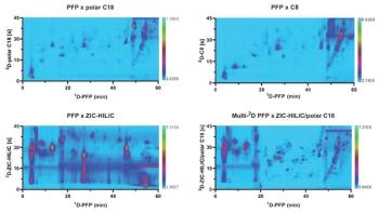
Calculation of the Surface Coverage as a Measure of Orthogonality: First of all, the surface coverage for the LC×LC separation of the 99-component standard mixture was calculated using the convex hull that includes all analyte spots (see Figure 4).

In this case, the convex hull is an eight-sided irregular polygon described by the points P1 to P8. The area of this convex hull was calculated by a vector method that Dück et al. used in their work (16). Accordingly, the area of the convex hull can be divided in six scalene triangles that are numbered in Figure 4. Each of these triangles can be described by two vectors that have the same corner point as origin and the other corner points as heads. The vectors that were used to determine the six areas are marked red in Figure 4. P1 was chosen as the origin of all vectors. The complete calculation can be found in reference 3. The surface coverage can now be approximated by the area ratio of the convex hull and the rectangular area, which is ~0.61 (or 61%). This result clearly underlines that both dimensions are only weakly correlated. According to Gilar et al., a coverage of 60% of the available separation space can be considered very high (4). The authors even state that for most practical applications a surface coverage higher than 63% cannot be achieved.

Comparison of 2D LC with 1D LC: A higher peak capacity is usually obtained in two‑dimensional liquid chromatography compared with one‑dimensional separations resulting in a higher number of compounds that can be chromatographically resolved. The user, however, is not primarily interested in whether it is possible to obtain a higher peak capacity. For practical purposes it is more important whether a two‑dimensional system will also lead to a significantly higher number of detected or identified compounds when compared to a one-dimensional separation. Therefore, the sample itself and not the theoretical peak capacity should be the basis for this evaluation. A direct comparison between a one‑dimensional and a two‑dimensional separation would be useful for an objective judgement of the performance of two‑dimensional separation approaches. However, there is only a very limited number of dedicated studies dealing with this issue (17). Leonhardt et al. recently made a comparison between a one‑dimensional and a two-dimensional chromatographic approach coupled to hybrid high‑resolution mass spectrometry (18). The comparison was based on a screening approach in environmental analysis, where three criteria for compound identification were employed. First, the accurate mass with a deviation of less than 5 ppm was used for identification. If the first criterion was fulfilled, the retention time should not deviate more than 2.5% from the retention time measured in the reference standard. If this criterion was also fulfilled, MS/MS spectra of the reference standard were compared with that of the sample. Figure 5 summarizes the results of this comparison.

All chosen compounds could be detected with both approaches on the basis of the accurate mass in the reference standard. When a real sample was analyzed, 48 compounds were found with the 1D LC approach, while 65 compounds could be detected with the miniaturized 2D LC approach. Using the retention time as an additional filter for the elimination of false positive hits, four compounds had to be removed in the 1D LC approach, while only one compound had to be eliminated for the 2D LC approach. It should be emphasized that retention time is a powerful parameter to ensure the identification of a compound. Of course, a further criterion for an unambiguous identification should be considered. MS/MS information can help to distinguish even isobaric compounds that have the same mass‑to-charge ratio, m/z. The possibility of acquiring additional MS/MS information also depends on the peak width. As can be seen from Figure 5, MS/MS information is only obtained for a small number of analytes that have been identified on the basis of the first and second criterion. The reason is that the algorithm for acquiring product ion spectra looks for the most intense peak in the full scan MS spectrum, which is then fragmented. Peaks with a lower intensity are not selected. Even if 10 MS/MS experiments are performed during one cycle, the compounds of interest might be missed because they possess an intensity too low compared to high abundant ions of the matrix. This could be circumvented if the algorithm is programmed that only ions of known substances are selected for fragmentation experiments. Nevertheless, the number of compounds that can be confirmed by applying all three criteria is significantly higher for the 2D LC approach. This demonstrates that the miniaturized LC×LC system performs well for screening purposes, although the absolute injection volume is reduced by a factor of 13 and a further dilution cannot be avoided by the modulation.

Solvent Consumption

The overall 2D solvent consumption of this miniaturized on-line LC×LC approach was compared to that of conventional fast 2D systems that use flow rates between 1 mL/min and 5 mL/min. While conventional fast 2D systems consume 1.44 L to 7.2 L of solvent over 24 h, only 0.0576 L are needed by a miniaturized 2D system operated at 40 μL/min. Keeping the rising solvent costs in mind, there are also reduced solvent costs when using miniaturized, on-line LC×LC systems compared with non‑miniaturized versions.

References

1. T.C. Schmidt, O.J. Schmitz, and T. Teutenberg, Analytical and Bioanalytical Chemistry 407, 117 (2015).
2. D.R. Stoll, J.D. Cohen, and P.W. Carr, Journal of Chromatography A 1122, 123 (2006).
3. J. Haun, J. Leonhardt, C. Portner, T. Hetzel, J. Tuerk, T. Teutenberg, and T.C. Schmidt, Analytical Chemistry 85, 10083 (2013).
4. M. Gilar, P. Olivova, A.E. Daly, and J.C. Gebler, Analytical Chemistry 77, 6426 (2005).
5. J. Leonhardt, T. Hetzel, T. Teutenberg, and T.C. Schmidt, Chromatographia78, 31 (2015).
6. E.L. Schymanski, H.P. Singer, P. Longree, M. Loos, M. Ruff, M.A. Stravs, C.R. Vidal, and J. Hollender, Environmental Science & Technology48, 1811 (2014).
7. Y.T. Li, J.S. Whitaker, and C.L. McCarty, Journal of Chromatography A1245, 75 (2012).
8. C. West, C. Elfakir, and M. Lafosse, Journal of Chromatography A1217, 3201 (2010).
9. S.Y. Wang, L.Z. Qiao, X.Z. Shi, C.X. Hu, H.W. Kong, and G.W. Xu, Analytical and Bioanalytical Chemistry407, 331 (2015).
10. G. Vanhoenacker and P. Sandra, Journal of Separation Science29, 1822 (2006).
11. T. Teutenberg, K. Hollebekkers, S. Wiese, and A. Boergers, Journal of Separation Science32, 1262 (2009).
12. D.R. Stoll, X.P. Li, X.O. Wang, P.W. Carr, S.E.G. Porter, and S.C. Rutan, Journal of Chromatography A 1168, 3 (2007).
13. F. Gritti and G. Guiochon, LCGC North America30, 586 (2012).
14. T. Teutenberg, S. Wiese, P. Wagner, and J. Gmehling, Journal of Chromatography A1216, 8470 (2009).
15. D.X. Li and O.J. Schmitz, Analytical and Bioanalytical Chemistry405, 6511 (2013).
16. R. Duck, H. Sonderfeld, and O.J. Schmitz, Journal of Chromatography A1246, 69 (2012).
17. Y. Wagner, A. Sickmann, H.E. Meyer, and G. Daum, J. Am. Soc. Mass Spectrom. 14, 1003 (2003).
18. J. Leonhardt, T. Teutenberg, J. Tuerk, M.P. Schlusener, T.A. Ternes, and T.C. Schmidt, Analytical Methods7, 7697 (2015).

Juri Leonhardt studied instrumental analytical chemistry and laboratory management and received his Ph.D. from the faculty of “Instrumental Analytical Chemistry” at the University Duisburg-Essen in 2016. Since 2011 he has been scientific coworker at the Institut für Energie‑ und Umwelttechnik e. V. (Institute of Energy and Environmental Technology) in Duisburg, Germany. His research is primarily focused on the development of miniaturized comprehensive multidimensional liquid chromatography systems based on nano- and micro‑liquid chromatography and their hyphenation to different detection techniques.

Jakob Haun studied water science at the University of Duisburg-Essen, Germany. From 2008 to 2012 he was a scientific coworker at the Institut für Energie- und Umwelttechnik e. V. in Duisburg. In 2014, he was awarded the Eberhard Gerstel Prize by the German Chemical Society (GDCh) and received his Ph.D. from the Faculty of Chemistry of the University of Duisburg-Essen. His related research was focused on the development of a multidimensional separation system for the qualitative screening analysis of complex samples (for example, wastewater). It is based on miniaturized on-line LC×LC hyphenated to quadrupole–time-of-flight mass spectrometry.

Torsten C. Schmidt is head of the Department of Instrumental Analytical Chemistry and the Center for Water and Environmental Research (ZWU) at the University of Duisburg-Essen, and scientific director at the IWW Water Centre in Mülheim an der Ruhr, Germany. He is currently president of the German Water Chemistry Society. In 2013, he received the Fresenius Award of the German Chemical Society. His main research interests include the development and application of analytical methods with a focus on separation techniques (GC, LC), sample preparation and compound‑specific stable isotope analysis, process‑oriented environmental chemistry, and oxidation processes in water technology.

Thorsten Teutenberg studied chemistry at Ruhr University Bochum, Germany. He studied for a doctorate in analytical chemistry at this institution, submitting a thesis on high-temperature HPLC. In 2004 his career took him to the Institut für Energie- und Umwelttechnik e. V. in Duisburg as a research associate. Since 2012 he has been in charge of the Research Analysis Department, mainly working on the various aspects of high-temperature HPLC, miniaturized separation and detection techniques, and multidimensional chromatography processes.

“Multidimensional Matters” editor Robert Shellie has extensive experience in hyphenated techniques. He joined Australian Centre for Research on Separation Science (ACROSS), University of Tasmania, Hobart, Australia, in 2005. He is currently Chromatography Market Manager at Trajan Scientific and Medical.